Location: Home >> Detail
J Acoust. 2019;1:e190003. https://doi.org/10.20900/joa20190003

1 Institute of Vibration, Shock and Noise, School of Mechanical Engineering, Shanghai Jiao Tong University, Shanghai, 200240, China
2 Key Laboratory of Aerodynamic Noise Control, China Aerodynamics Research and Development Center, Mianyang, 621000, Sichuan, China
3 Hagong Intelligent Robot Co., Ltd, Shanghai, 201100, China
* Correspondence: Weikang Jiang, Tel.: +86-21-34206332.
This article belongs to the Virtual Special Issue "Feature Paper"
Rolling element bearings are important parts of rotating machinery, and they are also one of the most fault-prone parts in rotating machinery. Therefore, many new algorithms have been proposed to solve the vibration-based diagnosis problem of rolling bearings. The measured vibration signal is typically composed of a periodic transient signal severely contaminated by loud background noise when the faults occur. In this paper, a transient signal extraction algorithm is proposed which depends on spectrum matrix decomposition. The sparse time–frequency representation of the periodic transient signals is exploited, and, further, a low-rank and sparse model is established to extract transient signals from strong noise. First, the low-dimensional representation matrix of the measured signal is generated by the synchrosqueezing transform based on short-time Fourier transform. It is found that the low-rank of the transient signal will be approximately preserved in the transformed domain. Then, semi-soft go decomposition is used to decompose the spectrum matrix into a low-rank matrix and a sparse matrix. Finally, the transient signal can be recovered through the inverse transformation of the decomposed low-rank matrix. The proposed method is a data-driven approach, and it does not require prior training. The performance of the algorithm is investigated on both synthetic and real vibration signals, and the results demonstrate that the algorithm is effective and robust.
Rolling element bearings are one of the most widely used components in mechanical systems, and their failure is one of the most frequent reasons for a machine breakdown [1]. Because of its low cost, high efficiency and convenient maintenance, it is widely used in the mechanical industry. It will cause a drop in the quality of the product when faults occur, or the bearings fail, and, in severe cases, it will lead to damage to the entire mechanical device. Therefore, considering the importance of bearings in mechanical equipment, fault diagnosis of bearings has caused widespread concern in the scientific community [2]. The ultimate goal of fault diagnosis is to determine the existence of the fault by analyzing the external fault information and determining whether the machine needs maintenance. Despite extensive research in the field, the diagnosis of these faults remains a challenging issue.
Vibration signal analysis has been extensively used in bearing fault diagnosis due to the simplicity of measurement and the relatively low cost of the sensor [3]. Generally, the presence of mechanical bearing faults can be detected by vibration signals analysis. From the literature research, diagnostic methods based on vibration signals analysis have proved their effectiveness in many situations, and researchers continually strive to develop improvements in the diagnostic algorithms based on vibration signals [4]. The defects of the rolling element bearings will produce a series of transient signals in the measured acceleration signal, as the fault repeatedly interacts with other rolling surfaces [5]. However, the measured vibration signals are always buried in background noise from other vibration sources on the machine, which results in the diversity and complexity of the vibration signal characteristics. Therefore, the detection and diagnosis of bearing faults can be considered as the problem of extracting periodic transient signals from the measured signals with strong noise.
In the past few decades, several methods for bearing fault diagnosis have been introduced and developed. These methods deal with vibration signals in a variety of ways and generally can be divided into the following categories [6].
Model-based methods: Models are used for enhancing the contrast between the fault signal and the normal vibration data. The most typical model-based approach is Autoregressive (AR) model, which is a time-sequence analysis method, and its parameters comprise essential information of the system condition [7]. AR model is widespread in machine fault detection and effective in extracting gear faults with little prior knowledge [8,9].
Spectral analysis methods: Spectral analysis methods aim to generate a spare time–frequency representation of the signal. The spectrum illustrates the characteristics of a signal in the time–frequency representation and presents more information than in the time domain. There are many ways to obtain the sparse time–frequency representation of the signal, such as short-time Fourier transform (STFT) and wavelet transforms [10–12]. Generally, fault signals and noise will show different properties in the time–frequency domain. It means that a sparse transform yields a more distinguishable representation. However, time–frequency transforms such as STFT and continuous wavelet transform spread the energy of the signal around the instantaneous frequencies of the original signal [13]. Hence, a post-processing method is proposed to sharpen the blurry signal information and to overcome the limitations of traditional time–frequency transforms. Synchrosqueezing transform (SST) utilizes frequency reassignment to shrink the spectrogram along the frequency axis, thus leading to a better resolution [14,15]. Therefore, SST can promote the sparsity of the representation matrix of the signal. Moreover, it is worth mentioning that SST is reversible.
Filtering methods: Filtering methods aim to reduce non-fault signals and enhance the visibility of the fault vibration. The fault information can be better revealed with the prior knowledge of the statistical characteristics of the fault signal. The most typical methods are presented, including Spectral kurtosis-based filtering and deconvolution. Spectral kurtosis (SK) is a method that selects a bandpass filter to maximize the kurtosis of the filtered resulting signal. SK has demonstrated its power in bearing fault diagnosis and has been receiving a lot of research attention within the last few years [16]. Minimum entropy deconvolution (MED) treats fault signal extraction as a deconvolution problem, in which a Finite Impulse Response (FIR) filter is selected to minimize the entropy of the filtered signal [17]. A limitation of MED is that the algorithm generally prefers to deconvolve only a single impulse, as opposed to the desired periodic impulses produced by bearing faults. Inspired by the MED deconvolution technique, an improved novel deconvolution norm was proposed, Correlated kurtosis (CK), which takes advantage of the periodicity of the faults [18]. The effectiveness of maximum correlated kurtosis deconvolution (MCKD) is proved by testing on the simulation and experimental data from a controlled gear tooth chip experiment.
Different from the previous work of building a matrix directly on the time domain and performing low-rank matrix decomposition [19], the present work depends on sparse time–frequency spectral analysis. The proposed method only requires that the signal has no information loss after the transformation, and the transformation is invertible. As mentioned above, the transform can capture the time–frequency structure of a periodic transient signal well. In this paper, the spectrum matrix of the measured signal is calculated using STFT-based SST due to its high resolution and high sparsity properties. It can be seen that the low-rank of transient signals will be approximately preserved during the transformation [20]. Then, the strategy is to decompose the matrix into low-rank and sparse components to obtain the transient signal corresponding matrix. Matrix factorization methods currently enjoy immense popularity in machine learning and signal processing [21]. There are many ways to obtain low-rank information from the noisy observation matrix with less error, such as robust principal component analysis (RPCA) [22,23] and go-decomposition (GoDec)[24].
The remainder of this paper is organized as follows. The signal model in bearing fault diagnosis and the STFT-based SST of signals are introduced in the Section “LOW DIMENSIONAL REPRESENTATION OF THE SIGNAL”. The selection of low-rank and sparse decomposition method is provided in Section “LOW-RANK DECOMPOSITION”. Then, Section “VALIDATION ON SYNTHETIC SIGNALS” presents the validation of the proposed methodology on synthetic signals. Finally, several actual vibration signals are used to verify the performance of the proposed approach in Section “VALIDATION ON VIBRATION SIGNALS”.
Typically, the measured signal y(t) can be described as the additive model,
y(t) = x(t) + n(t) (1)
where “informative signal” x(t) and the stationary background noise n(t) are assumed mutually independent. In the case of bearing fault diagnosis, the bearing components repeatedly strike the defect, resulting in periodic transient signals x(t).
The transient signal can be well captured in the time–frequency representation, on the contrary to the noise n(t), which is spread all over the time–frequency representation matrix [25]. It is found that different time–frequency transforms do not affect the extraction performance of transient signals through experiments. In this paper, based on the STFT of the signal, a sparser representation matrix is generated using SST.
The STFT expression of a function s ∈ L2(R) is defined as:

where g(t) is the window function with a unit norm ||g|| = 1.
Although the energy of the time–frequency representation Vf (η,t) diverges in the ridge direction, the phase of Vf (η,t) is not affected by the length of the time window, so the instantaneous frequency  can be estimated by the phase of Vf (η,t)[26,27].

In the actual calculation, η, t and ωf are discretized, i.e., Vf (η,t) is computed only at a discrete ak, with ak - ak-1 = (Δa)k, and its synchrosqueezed transform Tf(ω, t) is determined only at the center frequency ωl of successive bins [ωl - 1/2Δω, ωl + 1/2Δω], with Δω= ωl - ωl-1, by summing different contributions:

Finally, the signal x(t) can be reconstruction by the inverse transformation of Tf(ωl, t):

Let matrix X ∈  denote the STFT-based SST representation of transient signal x(t). The low-rank prior of the transient signal will be approximately preserved in the transformed domain, thus the spectrogram L = |X|2 is a low-rank matrix. Matrix Y ∈ is defined as the sparse time–frequency transform of the measured signal y(t) and the spectrogram M = |Y|2 can be represented as M = L + S. S corresponds to a stationary noise signal that is sparse. Therefore, by using the low-rank and sparse decomposition method, the noisy observation matrix can be decomposed to obtain the low-rank matrix, which containing transient signal information.
Without a constraint of specific rank, Robust Principal Component Analysis (RPCA) defines the low-rank component unclearly. Moreover, due to its convexity relaxation, the decomposed results sometimes are insufficiently promoted for low-rank or sparsity. As an improvement, in [24], the authors considered GoDec with a different signal model, M = L + S + R, with additive Gaussian noise R and penalizing constraints of rank and non-zero entries directly. Therefore, the problem of low-rank matrix and sparse decomposition can be formally expressed as,
M = L + S + R, rank(L) ≤ r, card(S) ≤ k (6)
where rank (L) is the rank of L, and card (S) is the cardinality of S. The problem in Equation (6) is approximately equivalent to solving the minimization of the following decomposition error:
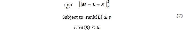
where the Frobenius norm 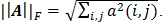 The optimization problem in Equation (7) can be solved by alternatively assigning the low-rank approximation of M − S to L and assigning the sparse approximation of M − L to S. Moreover, the singular value decomposition (SVD) is replaced with a Bilateral Random Projection (BRP)-based low-rank approximation, to significantly reduce the time cost [28,29](see Appendix A for details).
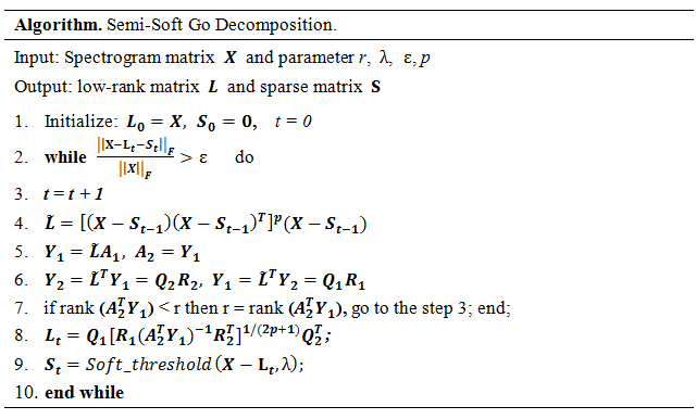
Generally, the cardinality of S is hard to estimate. Thus, Semi-Soft Go Dec (SSGD) adopts soft thresholding to the entries of S, where parameter can be automatically determined by soft threshold λ. Different from GoDec which imposes hard threshold to the entries of the sparse part S, card(S) can be relaxed by replacing it with the L1 norm 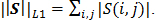 The value of regularization λ is the trade-off between the error term and the sparsity of S. Moreover, the computation cost of SSGD is substantially smaller than the original GoDec while the error rate is kept the same or even smaller. SSGD is formulated as the optimization problem in Equation (8), can be solved by the alternative optimization method, and the corresponding algorithm is presented in Appendix A.

Here, the convergence of SSGD needs to be discussed. Following the original GoDec [24], we can prove that SSGD can also converge to local optimum. The optimization problem in Equation (8) is equivalent to the following form.

Then, the optimization problem in Equation (9) can be solved by alternatively solving the following two subproblems until convergence:
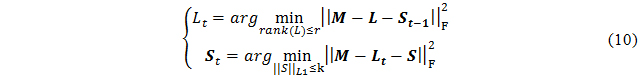
Let the objective value  after solving the two subproblems in Equation (10) be Et,1 and Et,2 in the tth iteration. Then, we have


The global optimality of St yields Et,1 ≥ Et,2 and the global optimality of Lt+1 yields Et,2 ≥ Et+1,1. Therefore, the objective values keep decreasing throughout Equation (10):
E1,1 ≥ E1,2 ≥ E2,1(13) ≥ ... ≥ Et,1 ≥ Et,2 ≥ Et+1,1 ≥ ... (13)
Since the objective of Equation (9) is monotonically decreasing, and the constraints are satisfied all the time, Equation (10) produces a sequence of objective values that converge to a local minimum.
Nevertheless, matrix L cannot be directly used to reconstruct the transient signal because the phase information is lost. The low-rank complex spectrum matrix can be recovered by taking over the phase information of matrix Y denoted by  and the sparse complex spectrum matrix is
  . It is noteworthy to point out that the spectrum matrix X is often contaminated by noise. Therefore, a binary time‐frequency mask method can be further used to refine the final results, which is written as follows:

where G is a parameter to control the amplitude gain ratio between |X(i,j)| and |N(i,j)|.
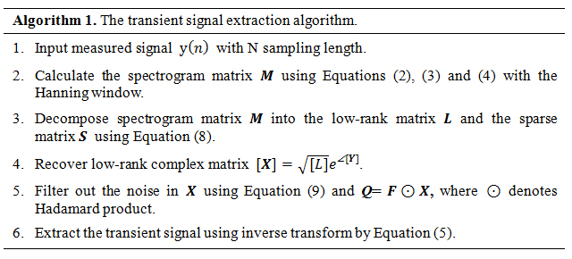
Finally, the estimated time–frequency spectrum of the signal can be transformed back to the time domain using the inverse transform. It is worth mentioning that the proposed method is very robust to STFT parameters and hyperparameter of SSGD according to the experimental verification. The transient signal extraction algorithm is shown in Algorithm 1. In addition, we give a guidance for parameter tuning in Appendix B.
In this section, we validate the proposed method with synthetic signals. We built the signal as a sequence of transients. It is monotonic and generated by x = s × h. Here, we use “×” to denote convolution, and s is an impulse train, as:
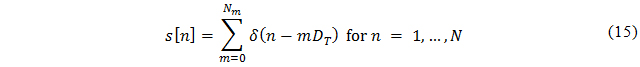
where δ(n) denotes the Dirac impulse, and h is a filter with the transfer function

Firstly, an impulse signal s[n] (time duration is 1 s and the sampling frequency is 104 Hz) with length N = 104 is produced, where DT = 600 and Nm = 16. Secondly, the impulse signal s[n] is passed through a filter H(z), with r = 0.95 to synthesize the transient signal x(n). Finally, Gaussian noise is added to the transient signal to obtain the simulated signal y(n) while maintaining the SNR = −10 dB. A simple illustrative example is shown in Figure 1, where the transient signal (in green color) is buried in strong additive noise (in blue color).
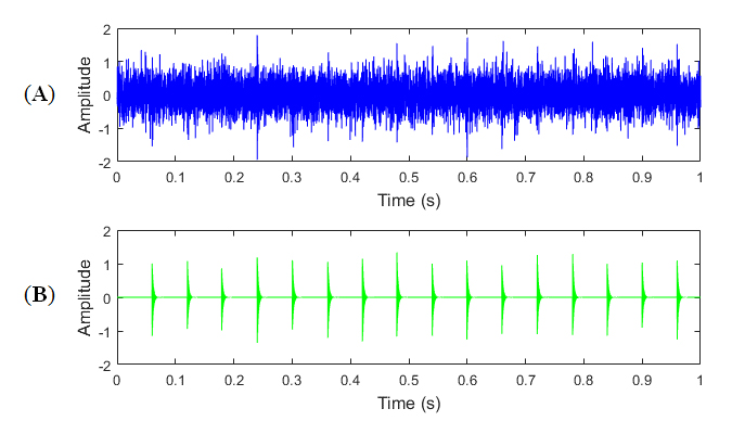 Figure 1. (A) A synthetic measured signal with white noise (SNR = −10 dB). (B) A synthetic periodic transient signal.
Then, a Hanning window with length Nw = 50 is selected for STFT-based SST, and the corresponding spectrogram of the raw signal and the transient signal are shown in Figure 2. It can be seen that the structure of the transient signal can be well captured after the transformation. On the contrary, the noise is spread over the entire time–frequency matrix. In other words, the low-rank of transient signal will not be actively changed after transform and can be considered as low-rank or semi-low-rank in the transformed domain. Therefore, the SSGD algorithm is used to decompose the spectrum of a raw signal into its low-rank and sparse components.
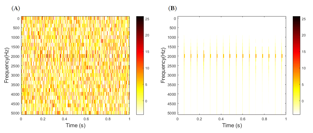 Figure 2. (A) Spectrogram of synthetic measured signal with a Hanning window with length Nw = 50 (SNR = −10 dB). (B) Spectrogram of the synthetic clean transient signal with Hanning window with length Nw = 50.
In this case, two important parameters in the SSGD is set to r = 1 and λ = 0.02. It is found that the decomposed low-rank and sparse spectrum can be attributed to the synthetic transient signal and the noise, respectively, as shown in Figure 3. However, there are differences between the extracted low-rank spectrum and spectrogram of the clean synthetic transient signal. These differences come from the fact that the transient signal in the time–frequency domain is not exactly low-rank, but it would be approximately low-rank. Therefore, the decomposed low-rank matrix can still be used to reconstruct transient signals.
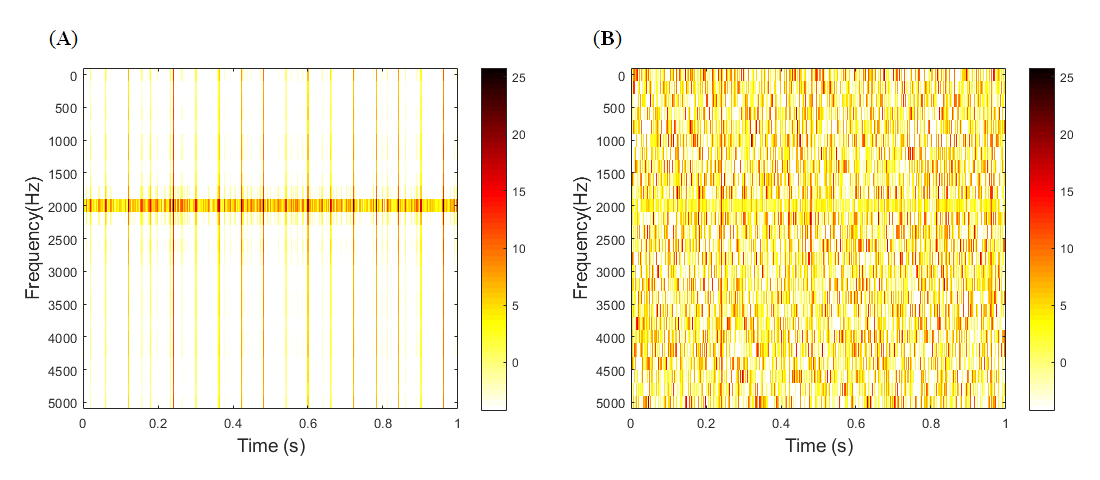 Figure 3. (A) Low-rank spectrum decomposed by SSGD algorithm with r = 1 and λ = 0.02. (B) Sparse spectrum decomposed by SSGD algorithm with r = 1 and λ = 0.02.
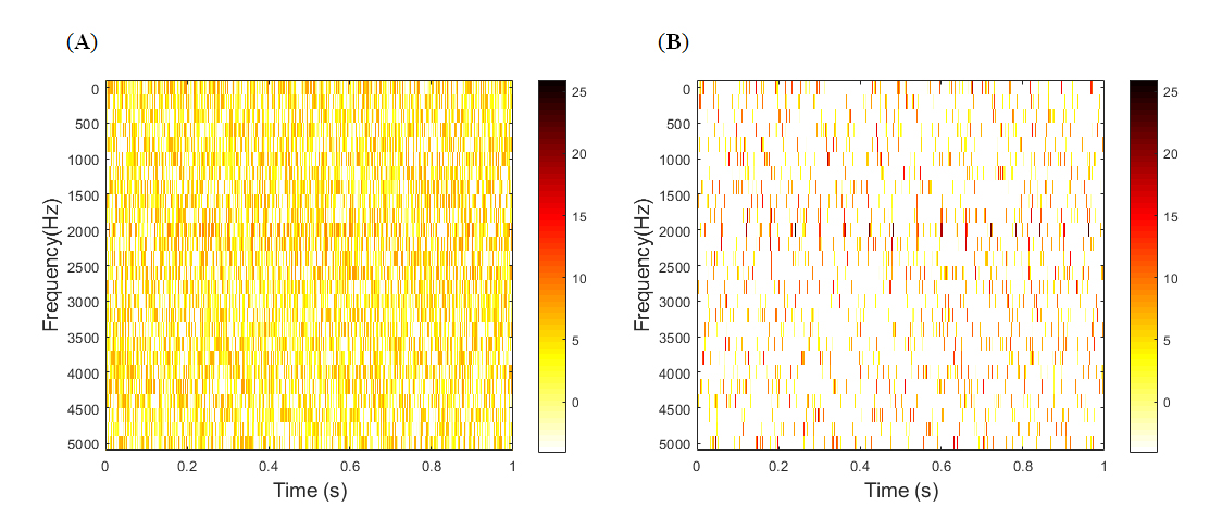 Figure 4. (A) Low-rank spectrum decomposed by RPCA algorithm with λ = 0.02. (B) Sparse spectrum decomposed by RPCA algorithm with λ = 0.02.
Similar to the previous work using RPCA for low-rank decomposition [30], here, RPCA is used to decompose the STFT-based SST spectrum and the results are presented in Figure 4. It is not easy to determine whether the transient signal is in the low-rank or the sparse component, compared with Figure 3. Further, the singular values of the decomposed matrices are calculated to test the validity of low-rank and sparse decomposition algorithm. Distributions of singular values of the decomposed low-rank and sparse matrix by SSGD and RPCA are displayed in Figure 5. It can be found that the rank of the low-rank matrix obtained by RPCA is even larger than the sparse matrix. The reason for this may be the convex relaxation of RPCA. Due to its convexity relaxation, the decomposed results are insufficiently promoted for low-rank or sparsity. On the contrary, the low-rank matrix decomposed by SSGD satisfies its definition well just because the algorithm imposes a hard constraint on the rank. Besides, SSGD is significantly less time-consuming than RPCA.
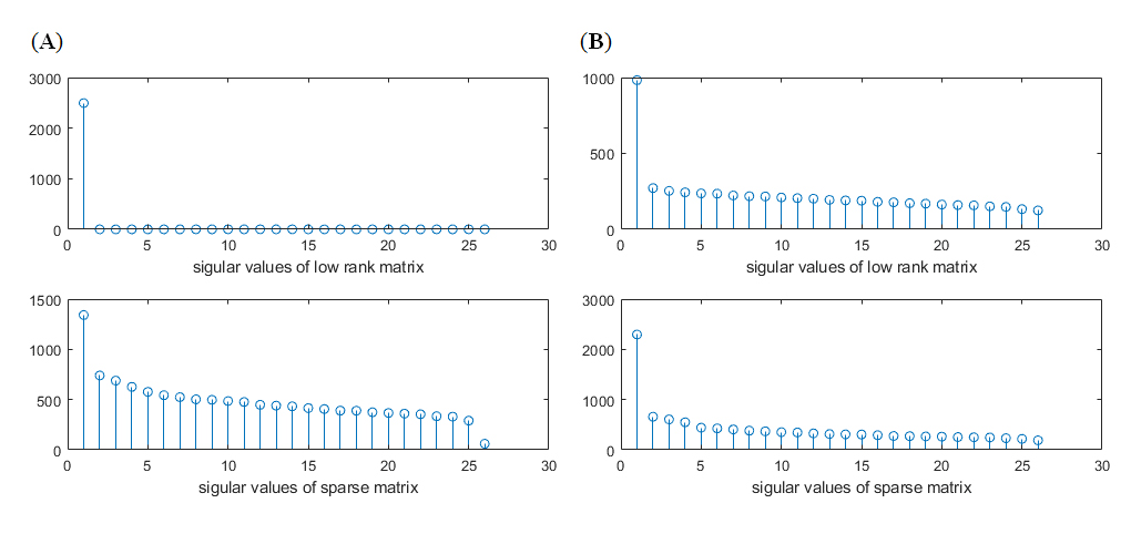 Figure 5. (A) Distribution of singular values of the decomposed low-rank and sparse matrix by SSGD.
(B) Distribution of singular values the decomposed low-rank and sparse matrix by RPCA.
Figure 5. (A) Distribution of singular values of the decomposed low-rank and sparse matrix by SSGD.
(B) Distribution of singular values the decomposed low-rank and sparse matrix by RPCA.
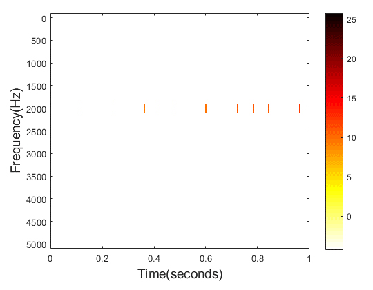 Figure 6. Filtered low-rank spectrum matrix Q = F ⊙ X with G = 6.
Then, the phase information of the raw signal spectrum is used to recover the low-rank complex spectrum. A binary time‐frequency mask is used to remove noise to obtain a more accurate low-rank spectrum. The filtered low-rank complex spectrum Q = F ⊙ X is presented in Figure 6. Compared with Figure 2B, it is found that the result is good with the clean transient signal spectrum.
Finally, the estimated filtered low-rank spectrum matrix can be transformed back to the time domain using the inverse STFT-based SST, to obtain the transient signal, which is presented in Figure 7C. It can be seen that the periodic transient signals are almost entirely recovered, compared with Figure 7A,B, which proves the effectiveness of the proposed method.
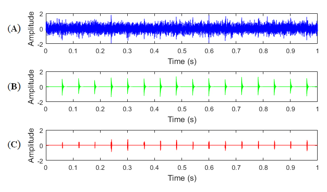 Figure 7. (A) A synthetic measured signal with white noise (SNR = −10 dB). (B) A synthetic periodic transient signal. (C) The extracted transient signal by our proposed method (Figure 6 shows that only 10 transients are recognized because the other values are too small to display).
In addition, there are many methods to recover sparse transients from noise. To emphasize the advantage of the low-dimensional modeling of fault signal, a Matching Pursuit (MP) based algorithm is used for comparison [31]. The crucial step of MP-based algorithms is the establishment of a sparsity-promoted dictionary, and the majority of known ways for establishing a dictionary can be divided into two general categories: analytic- and learning-based approaches [31]. An important issue is that such an analytic dictionary always needs to be established in advance, which inevitably causes the effect of extraction to be greatly affected by the dictionary. Often, in practical applications, it is very difficult to choose and build a dictionary properly.
Figure 8 shows the extraction of transient signals by the MP algorithm. It can be found that both methods can capture the time of transient signal well, but the transient signal extracted by the MP-based algorithm is still mixed with some noise, and the proposed method performs well in noise reduction. In comparison, our method requires only a small number of parameters to achieve good results, and the method is robust to parameters.
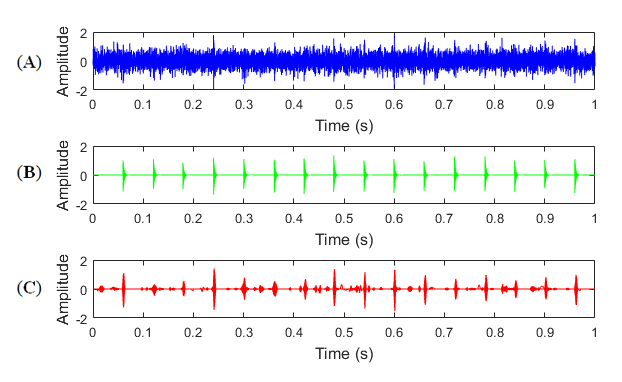 Figure 8. (A) A synthetic measured signal with white noise (SNR= −10 dB). (B) A synthetic periodic transient signal. (C) The extracted transient signal by MP-based method.
This section illustrates the application of the proposed method on actual vibration signals, as often encountered in industrial applications. The rolling bearing experimental data are from the MFPT Challenge data [32], which comprises data from a bearing test rig (nominal bearing data, an outer race fault at various loads, and inner race fault and various loads). A fault is mainly identified by estimating the fault frequency and associating it to a given component in the machine. The prevailing method in the modern literature is surely the squared envelope spectrum, which reveals the repetition frequency of the transient signal series [33]. The following shows the application of the proposed method and envelope spectrum analysis in real vibration data.
As for inner race fault, the expected components in the envelope spectrum are ball pass frequency inner race (BPFI) and its harmonics, and sidebands spaced at shaft speed and their harmonics [5]. The envelope spectrum of the raw inner race fault shows that most of the energy is focused on BPFI and its harmonics, as shown in Figure 9. It indicates an inner race fault of the bearing, which matches the fault type of the signal. Therefore, the type of bearing fault can be detected by envelope spectrum analysis. Figure 10A indicates that the inner race fault signal has significantly larger impulsiveness in the time domain, making envelope spectrum analysis capture the fault signature at BPFI effectively.
Then, the extracted transient signal by the proposed method is displayed in Figure 10B, which approximately captures the time position of the transient signal. Besides, the envelope spectrum of the extracted transient signal by the proposed method is presented in Figure 11. It is also found that most of the energy is focused on BPFI and its harmonics, which indicates the fault type of the signal. Moreover, the proposed method captures the sidebands in the low-frequency region better than the envelope spectrum directly on the raw signal. It also proves that the proposed algorithm is very effective in diagnosing fault types.
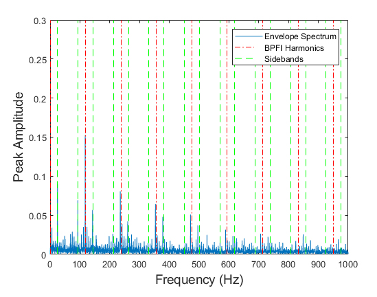 Figure 9. Envelope Spectrum of the raw inner race fault signal, the expected BPFI and its harmonics (red dashed line) and the expected sidebands (green dashed line).
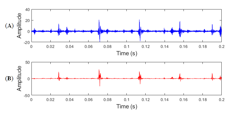 Figure 10. (A) The raw inner race fault signal data. (B) The extracted transient signal by the proposed method.
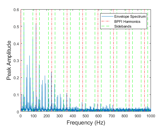 Figure 11. Envelope Spectrum of the extracted transient signal by the proposed method.
The expected components in the envelope spectrum are ball pass frequency outer race (BPFO) and harmonics of an outer race fault signal. Therefore, most of the energy in the envelope spectrum of the outer race signal should be concentrated at BPFO. However, it is found that there are no clear peaks at BPFO harmonics when the raw signal envelope spectrum is analyzed, as shown in Figure 12. It illustrates that envelope spectrum analysis on the raw signal does not provide useful diagnostic information. The outer race fault signal does not have a significantly larger impulsiveness, and it is masked by the loud noise, as shown in Figure 13A, making envelope spectrum analysis unable to capture the fault signature at BPFO effectively. Therefore, the raw signal needs to be preprocessed to extract the transient signal under strong signal before envelope spectrum analysis. Here, the proposed method is used for preprocessing, and the extracted transient signal is shown in Figure 13B.
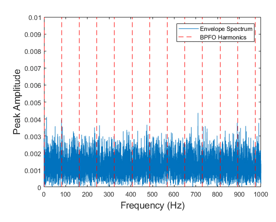 Figure 12. Envelope Spectrum of the raw outer race fault and the expected BPFI and its harmonics (red dashed line).
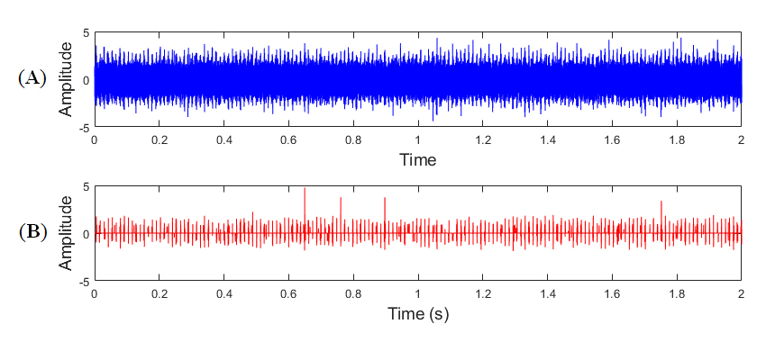 Figure 13. (A) Raw outer race fault signal. (B) The extracted transient signal by the proposed method.
Further, envelope spectrum analysis is carried out for the extracted transient signal, as shown in Figure 14A. It can be seen that there is a significant peak at BPFO, compared with Figure 12, which proves that the proposed preprocessing method is very useful for the extraction of fault information. Moreover, the envelope spectrum of the transient signal extracted by the proposed algorithm is compared with SK algorithm, as presented in Figure 14. It is found that the proposed method captures fault information well in high-frequency harmonics compared to the SK method. It further demonstrates the effectiveness of the proposed method in the diagnosis of vibration fault signals.
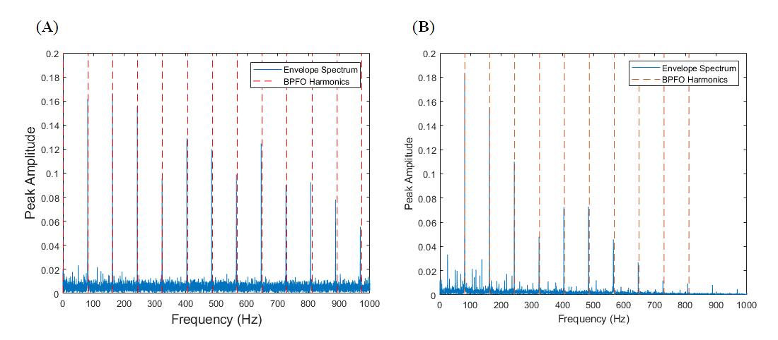 Figure 14. (A) Envelope Spectrum of the extracted transient signal by the proposed method. (B) Envelope Spectrum of the signal by SK algorithm.
This paper has introduced a low-dimensional model for the vibration signal of rolling element bearing faults, which has the typical form of a series of transients overlaid with stationary background noise. It is based on the sparse representation of the signal and the characteristics of transient signals expressed in a sparse representation. In this work, STFT-based SST is utilized to transform the noisy measured signal to the high-resolution time–frequency domain. The low-rank of the transient signal will be preserved in the transformed domain. The filtered transient signal can be recovered through the inverse transformation of the low-rank component of the SST magnitude spectrum, which is obtained by solving the optimization problem using the Semi-Soft GoDec algorithm. This paper aims to exploit the low-dimensional model of periodic transient signals and establish a low rank and sparse model for fault detection of bearings. The performance of the proposed method has been tested on several synthetic signals and real vibration signals. In terms of reconstruction of the fault signal, results demonstrate that the method is effective and robust. The proposed model also deals with signals acquired from the actual vibration machine. The advantage of the proposed method is that it does not require prior training or other particular features and only requires the setting of a few parameters.
LY conceived the method and carried out the derivation procedure. WD wrote the manuscript and finished the simulation and experimental validation. SH validated the formulations and participated in drafting the manuscript. WJ coordinated the research. All authors gave final approval of the version to be submitted.
The authors declare that they have no conflicts of interest.
This work was supported by the National Natural Science Foundation of China (Grant No. 11704248, 51835008, 11574212) and the Open Fund of the Key Laboratory of Aerodynamic Noise Control (ANCL20180302).
The authors would like to thank the continuous support from Prof. Jerome Antoni and Prof. Quentin Leclere (Laboratoire Vibrations Acoustique, INSA de Lyon).
Fast low-rank approximation [24]:
Given r bilateral random projections (BRP) of an m × n dense matrix X, i.e., Y1 = XA1 and Y2 = XT A2, wherein A1 ∈  and A2 ∈
  are random matrices, L = Y1(A2T Y1)-1 Y2T is a fast rank-r approximation of matrix X. When singular values of X decay slowly, L may perform poorly. A modification for this situation based on the power scheme is used. In the power scheme modification, we instead calculate BRP of a matrix X ̃= (XXT)p X, whose singular values decay faster than X. To obtain the approximation of X with r, we calculate the QR decomposition of Y1 and Y2, i.e., Y1 = Q1R1, Y2 = Q2R2. Therefore, the low-rank approximation of X is
 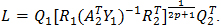 In addition, the power scheme modification reduces the error of low-rank approximation by increasing p. In this paper, the values of p are all set to 6.
A soft thresholding operator for any matrix Q is defined as:
Soft_threshold(Q, λ) = max(|q| - λ, 0) sgn(q)
where q denotes each entry of the matrix Q and sgn() is the sign function.
Parameter (r, λ, G) selection strategy:
1.
2.
3.
1.
2.
3.
4.
5.
6.
7.
8.
9.
10.
11.
12.
13.
14.
15.
16.
17.
18.
19.
20.
21.
22.
23.
24.
25.
26.
27.
28.
29.
30.
31.
32.
33.
Yu L, Dai W, Huang S, Jiang W. Sparse Time–Frequency Representation for the Transient Signal Based on Low-Rank and Sparse Decomposition. J Acoust. 2019;1:e190003. https://doi.org/10.20900/joa20190003

Copyright © 2020 Hapres Co., Ltd. Privacy Policy | Terms and Conditions


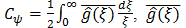 is the complex conjugate of the Fourier transform of ĝ(ξ).