ABBREVIATIONS

LB, Late Blight; Rgene, gene of resistance; Pi, Phytophthora infestans; AVR, avirulence gene.

INTRODUCTION

Late blight (LB) is one of the most devastating diseases in potatoes, tomatoes, and tobacco. It is caused by an oomycete called Phytophthora infestans (Pi), which can attack all parts of the plant. An infection by this pathogen can result in complete destruction of the plant in a few days. Pi originated from Peru and Mexico and was most likely introduced to Europe in the mid XIXth century along with contaminated potatoes imported from North America in order to fight another disease. Subsequently, LB was partially the cause of the famine in Europe in the XIXth century, that in particular hit Ireland [1]. From this point, massive efforts were conducted to fight LB, going from the development of fungicides, management recommendations, and development of resistant lines through screening for natural resistance in established potato varieties as well as in wild potatoes [1]. The consequences of LB and of the control measures taken were in 2009 estimated to cost €9 billion worldwide [2]. This cost included the loss due to LB contamination, the cost of the fungicides and many other factors such as the societal cost, including for example the impact on human health. While having an important cost, the use of fungicides is widely preponderant to fight LB. In 2016 in the Netherlands, the amounts of fungicides used against LB represented 50% of the total amount of pesticides used [3]. Besides their economic and societal costs, with time, some fungicides became inefficient as Pi evolved to become resistant to the treatments. One of the latest examples is the LB genotype EU43 which to is resistant to mandipropamid [4].

Another way to fight LB is by establishing new genetic resistance. Following the mid-XIXth century crisis, intensive work was done especially in the early XXth century to identify wild potatoes which were resistant to LB and the genes responsible for this resistance [5]. It is assumed that the resistance of a host to a pathogen relies on the interaction of a gene of resistance (Rgene) expressed in the host and an avirulence gene (AVR gene) expressed in the pathogen [6]. Those two genes presumably co-evolved simultaneously and, therefore, the plants and the pathogens carrying the matching pairs of Rgenes and AVR genes originate from the same geographic regions. This phenomenon is the reason why primary sources of resistance to Pi were searched for in wild populations of Solanum spp. in South America and Mexico. Over 70 genes of resistance to Pi has now been recognized as identified in wild Solanum species and as well as some in cultivated potatoes Solanum tuberosum [7,8]. This has led to the development of varieties showing higher resistance. However, here again, because of its ability to evolve, Pi can escape the resistance conveyed by incorporated Rgenes. Indeed, the introgression of eleven dominant resistant genes first identified in Solanum demissum L. (R1–R11) did not lead to long term resistance to Pi [9]. Moreover, while some resistance genes such as Rpi-blb3 [10] or the Rpi2 locus [11] confer resistance toward a large spectrum of pathotypes while others such as R3a, R3b, R6 and R7 [12,13] confer a resistance only to specific pathotypes. One of the strategies proposed to slow down the ability of the pathogen to escape resistance is to stack several Rgenes in one cultivar [14]. However, such R-genes need a broad spectrum of resistance in order to ensure long term resistance. Introgression of two or three resistance genes through traditional breeding is a lengthy process. It took half a century to get two new varieties of S. tuberosum carrying Rpi-blb2 coming initially from S. bulbocastanum [3]. The difficulty in introgression also depends on the endosperm balance number (EBN) that determines the ease of crossing related potato species. Different methods such as hybrid breeding and genetic engineering could be used to stack Rgenes more efficiently in cultivated potato. Some studies have used such technologies and were able to stack up to 4 Rgenes into S. tuberosum [3,15–17], leading to plants being highly resistant to LB. In theory, if a single clone carried the advantageous allele for four R-genes, it would be nearly impossible for the pathogen to overcome this resistance [18]. However, this relies on prerequisites such as that the R-genes should be 100% effective, which most likely is unrealistic. Moreover, currently, the deployment on the European market of varieties developed using genetic engineering is limited. We should also consider if resistance should only rely on the Rgenes or whether genetic variation in the polygenic background is of importance for resistance to LB. In a recent review McGee et al. [19] argued that use of identified R-Genes needs to be combined with quantitative disease resistance, often based on many minor genes, because resistance due to specific genes the tends to vane over time due to strong selection on the disease agents.

Creating lines resistant to LB through breeding is a possibility to avoid crop destruction by the disease and reduce the current reliance on pesticides. This is also reflected in the general strategy for the International Potato Center (CIP) [20]. Heritability estimates for LB resistance reported in literature ranged from 0.31 to 0.85 [21–25], which suggests that selection for LB resistance can be very effective. One of the challenges for selecting for LB resistance has been to be able to improve resistance without negatively impacting other traits of economic importance. One example is maturity, for which it has been observed that cultivars selected for LB resistance showed late maturity. It has been shown that QTLs for blight resistance and QTLs for maturity were found at same position [26,27].

Traditional genetic improvement in potatoes has been slow due to the need for extensive testing in multiple environments and the low multiplication rate due to the vegetative formation of clones. However, the genetic constitution of clones is fixed after the first crossing generation and this, combined with extensive genotyping in early multiplication generations, can lead to genomic predictions of line performance before large scale multi environmental trails (METs) can be conducted. If genotyping is sufficiently cost effective this can lead to a remarkably high selection intensity and short generation intervals.

The lack of persistent resistance toward Pi as discussed above is due to constant development in the disease agent. The Euroblight network monitors the rapid evolution of Pi across the main potato growing regions in Europe. Clearly there are major time-dependent changes in the dominant Pi populations. Yearly reports on results of this monitoring can be found at https://agro.au.dk/forskning/internationale-platforme/euroblight (accessed on 20 July 2023) [28]. Long term testing of resistance will enable monitoring development in resistance over time and to estimate the genetic correlation between resistance measured at separate times. This will indicate the combined effect of evolution of the disease agent and the effects of potential selection for resistance for LB in potato. To our knowledge such analysis has not been attempted before.

In the period investigated the breeding program mostly was based on sequential phenotypic selection on disease traits in early clonal generations, and later selection on maturity, yield, and quality traits. If genetic correlations between early recorded traits and later yields traits are negative this may lead to limited genetic progress because advances in early selection steps are counteracted by selection in later steps due to negative relationships between early and late recorded traits.

The aims of our study were to estimate the heritability for LB resistance in a Danish potato population and search of quantitative trait loci with large effects in order characterize the genetic architecture of LB resistance in potato and to develop genomic based selection criteria for LB resistance, where both identified genome areas carrying disease resistance and quantitative disease resistance based on many minor genes are exploited to increase resistance to LB. In addition, we aim to evaluate the genetic development of LB resistance over longer time periods.

MATERIAL AND METHODS

The tested plants were all parts of the routine breeding program run by Danespo A/S. Early in the breeding program wild relatives were crossed into the population and in more recent years markers have been used for early selection and genes stacking. Historically, selection in the population has primarily been based on phenotypic records from inoculated field trials. The same testing procedure for LB resistance has been used throughout the period investigated.

Every year new parents were selected and crossed. Seeds were grown per family in the green house and at an early stage moved to individual pots. A single tuber from each individual pot was grown in the field for replication. In following years tubers from individuals of interest were tested for LB resistance. There were no clones that did not stem from the routine breeding program. The criteria for selecting parents have changed over the years but is not expected to influence results reported here. The plant material stem from a total of 36 years of crossing new parents. In early years only a few progenies of selected parents were tested but in later years a large group of clones were included (Table 1). This reflects a gradual increase in the importance of LB resistance in the breeding program.

TABLE 1

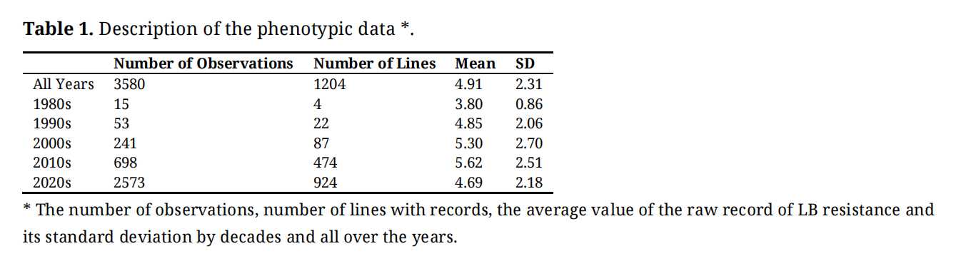Table 1. Description of the phenotypic data *.

The resistance to Pi was phenotyped by exposing the plants to an isolate of the disease agent collected in Denmark the year preceding the resistance test. Tests for disease resistance were performed for 36 consecutive years and, therefore, different pathotypes of Pi were used. However, no systematic characterization of the pathotype was carried out, but it must be expected that the dominant pathotype has changed over the years. (Euroblight, https://agro.au.dk/forskning/internationale-platforme/euroblight) (accessed on 20 July 2023) [28]. The test trial was designed by alternating one infector row and two test rows. The infector row was a mix of Bintje, which is a highly susceptible variety and was used across all the 36 years of test, and 2 other susceptible varieties that varied over time. On all four sides of the trial, there was an infector row. Each plot consisted of three plants with a distance of 33 cm, and each plot was 75 cm away from each other. The resistance to LB was assessed by attributing a grade to each plot, constituting three plants, based on foliage observation. The grades ranged from 1 (dead plant) to 9 (no sign of infection). A grade of 2 meant that only 0.1% to 4% of the green leaves remained, and the stems were fully attacked. For a grade of 3, 5% to 14% of the leaves were still green and the stems were also attacked. When 15% to 39% of the leaves were green and the stems were attacked, it was given a grade 4. Grade 5 meant that 40% to 59% of green leaves persisted, with the stems still being affected. If 60% to 70% of the leaves were green but the stems remained untouched, it was given a grade of 6. Grade 7 was given when only 5 to 10 leaves showed infection, and finally, grade 8 signified just 1 to 2 leaves were infected. This definition corresponds to scoring for resistance toward LB which is common among breeders. Papers focusing on epidemiology tend more often to use a reversed scale and then denoting it susceptibility. A full description of the scores is given in [29].

Sample DNA from 1628 varieties were genotyped using a custom 10k Affymetrix chip (10647 SNP). Genotyping was done over two batches, with five lines being genotyped in both batches. Fifteen SNP markers showing inconsistent genotypes in more than three of the five lines genotyped in both years were discarded. Then, only one genotype record was kept for further analyses of the duplicated genotypes. Next, 1108 SNP were excluded for having a call rate lower than 50%. No individuals were excluded based on an individual call rate lower than 40%. At the end, the genotype dataset used for analysis consisted of 1628 individuals genotyped for 9524 SNP. Finally, missing values were imputed using a random forest approach [30] with 50 trees using the missRanger R package [31].

The genomic map used to find the location of significant SNPs is the map corresponding to the DM v6.1 assembly [32]. The SNPs were mapped on the twelve chromosomes of potato, and a group of SNPs that had an unassigned position on the genome.

Different univariate models were evaluated to find the best fitting model.

y = Xb + Za + e (1)

y = Xb + Za + Wp + e (2)

y = Xb + Za + Egxd + e (3)

Where X, Z, W and E are the incidence matrices for fixed effects, the additive genetic effect, the non-additive genetic effect and the genotype by decade of testing interaction effect, respectively. The vector b of the fixed effects included market segment, genotyping batch, and year of the challenge test. The vectors a, p, gxd and e are vectors of the additive genetic effect, the non-additive genetic effect, the genotype by decade interaction effect and the residual environmental effect, respectively. For the interaction, the decades were built on the year of the challenge test and so we had five decades; 1980s, 1990s, 2000s, 2010s and 2020s. The effect of p was left out of model (3) because the corresponding variance component converged toward zero. The distributional assumptions were $<b\; style="\; font-weight:bold">a</b>~\text{N}[0,A{\text{σ}}_{\text{a}}^2]$ , $<b\; style="\; font-weight:bold">p</b>~\text{N}[0,I{\text{σ}}_{\text{p}}^2]$ , and $<b\; style="\; font-weight:bold">gxd</b>~\text{N}[0,I{\text{σ}}_{\text{gxe}}^2]$ . Where A was the pedigree-based relationship matrix for all clones, and I is an identity matrix of size corresponding to the number of individuals in p and the number of genotype by decade interaction effects for gxd. The pedigree-based relationship matrix was computed using the “AGHmatrix” package in R [33] assuming a ploidy of four and a probability of occurrence of double reductions of 0.005.

A multivariate (MT) model was used to estimate the (co)variance components for the three decades, for which more than 100 observations were available. In this case, there are three phenotypes, LB₀₀, LB₁₀ and LB₂₀ which are the phenotypes of the resistance to LB for tests done in 2000s, 2010s and 2020s, respectively. Only the phenotypes of those decades were kept because the few observations available for the early decades lead to convergence issues.

$\left[\begin{array}{c}{\text{<b style=" font-weight:bold">LB</b>}}_{\text{<b style=" font-weight:bold">00</b>}}\\ {\text{<b style=" font-weight:bold">LB</b>}}_{\text{<b style=" font-weight:bold">10</b>}}\\ {\text{<b style=" font-weight:bold">LB</b>}}_{\text{<b style=" font-weight:bold">20</b>}}\end{array}\right]$ $=$ $\left[\begin{array}{c}{\text{<b style=" font-weight:bold">X</b>}}_{\text{<b style=" font-weight:bold">00</b>}}\\ 0\\ 0\end{array}\begin{array}{c}\text{0}\\ {\text{<b style=" font-weight:bold">X</b>}}_{\text{<b style=" font-weight:bold">10</b>}}\\ \text{0}\end{array}\begin{array}{c}\text{0}\\ \text{0}\\ {\text{<b style=" font-weight:bold">X</b>}}_{\text{<b style=" font-weight:bold">20</b>}}\end{array}\right]$ $\left[\begin{array}{c}{\text{<b style=" font-weight:bold">b</b>}}_{\text{<b style=" font-weight:bold">00</b>}}\\ {\text{<b style=" font-weight:bold">b</b>}}_{\text{<b style=" font-weight:bold">10</b>}}\\ {\text{<b style=" font-weight:bold">b</b>}}_{\text{<b style=" font-weight:bold">20</b>}}\end{array}\right]$ $\left[\begin{array}{c}{\text{<b style=" font-weight:bold">Z</b>}}_{\text{<b style=" font-weight:bold">00</b>}}\\ 0\\ 0\end{array}\begin{array}{c}\text{0}\\ {\text{<b style=" font-weight:bold">Z</b>}}_{\text{<b style=" font-weight:bold">10</b>}}\\ \text{0}\end{array}\begin{array}{c}\text{0}\\ \text{0}\\ {\text{<b style=" font-weight:bold">Z</b>}}_{\text{<b style=" font-weight:bold">20</b>}}\end{array}\right]$ $\left[\begin{array}{c}{\text{<b style=" font-weight:bold">a</b>}}_{\text{<b style=" font-weight:bold">00</b>}}\\ {\text{<b style=" font-weight:bold">a</b>}}_{\text{<b style=" font-weight:bold">10</b>}}\\ {\text{<b style=" font-weight:bold">a</b>}}_{\text{<b style=" font-weight:bold">20</b>}}\end{array}\right]$ $+\text{<b style=" font-weight:bold">e</b>}$ (4)

Where X₀₀, X₁₀, X₂₀, Z₀₀, Z₁₀ and Z₂₀ are the incidence matrices for the fixed effect and the additive genetic effect. b is the vector of the fixed effect, which are market segment, the genotyping batch, and the year of the challenge test. The vectors a_xx, and e were the additive genetic effect and the residual environmental effect, respectively,

$\text{with}\left[\begin{array}{c}{\text{<b style=" font-weight:bold">a</b>}}_{\text{<b style=" font-weight:bold">00</b>}}\\ {\text{<b style=" font-weight:bold">a</b>}}_{\text{<b style=" font-weight:bold">10</b>}}\\ {\text{<b style=" font-weight:bold">a</b>}}_{\text{<b style=" font-weight:bold">20</b>}}\end{array}\right]~\text{MVN}\left[[\mathrm{<b\; style="\; font-weight:bold">0</b>},\mathrm{<b\; style="\; font-weight:bold">A</b>} \otimes \left(\left(\begin{array}{ccc}\begin{array}{c}{\text{σ}}_{{\text{a}}_{00}}^2\\ {\text{σ}}_{{\text{a}}_{00}{\text{a}}_{10}}\\ {\text{σ}}_{{\text{a}}_{00}{\text{a}}_{20}}\end{array}& \begin{array}{c}{\text{σ}}_{{\text{a}}_{00}{\text{a}}_{10}}\\ {\text{σ}}_{{\text{a}}_{10}}^2\\ {\text{σ}}_{{\text{a}}_{10}{\text{a}}_{20}}\end{array}& \begin{array}{c}{\text{σ}}_{{\text{a}}_{00}{\text{a}}_{20}}\\ {\text{σ}}_{{\text{a}}_{10}{\text{a}}_{20}}\\ {\text{σ}}_{{\text{a}}_{20}}^2\end{array}\end{array}\right)\right)]\right]$

The (co)variance components in all models were estimated by REML using the AI-REML procedure in the DMU software package [34].

Narrow sense heritability (h²) estimates were computed, as the estimated additive genetic variance divided by the estimated phenotypic variance and presented in tables as relative variance due to additive genetic effects. Similarly, the proportion of non-additive genetic variance was presented as the relative genetic variance due to non-additive effects. The broad sense heritability (H²) is then the sum of the relative variance due to additive and due to non-additive genetic effects. The estimated phenotypic variance was computed as the sum of all the estimated variance components for each model. Therefore, both narrow sense and broad sense heritability refer to an individual measurement from a plot consisting of three plants and do not refer to the heritability of variety means because the amount of replication varies.

The effect of each SNP (from 1 to 9524) was estimated using single marker regression using a SNP-by-SNP approach (step 1). If at least one significant SNP was found on the genome, the genotype of the most significant SNP, referred to as the Top-SNP, was added to the model as a fixed effect (step 2), and GWAS were run again.

step 1 => y = Xb + β*SNP_i + Za + Egxd + e (5)

step 2 => y = Xb + β_T*Top-SNP + β*SNP_i + Za+ Egxd + e (6)

The first step of model 5 is like model 3. The only difference is the addition of a regression on an individual SNP. β is the effect of SNP_i. In step 2, the genotype of the most significant SNP identified across the genome in the first step was added as a fixed effect to the model (Top-SNP). This process was repeated until no more significant SNP were identified. The significance threshold was set at 0.05/9524 = 5.25 × 10⁻⁶ based on the Bonferroni correction.

A QTL with significant effect on LB resistance was defined as a SNP or a group of SNPs capturing the same effects on LB. The group of SNPs were defined using model (6) in the two-step procedure of the GWAS. Each group of SNPs were represented by only the most significant SNP, referred as the Top-SNP. Model (5) was rerun with all Top-SNP included as fixed effects to estimate the remaining additive genetic variance. The relative amount of additive genetic variance explained by the chromosome region were then expressed as the reduction in additive genetic variance from model (6) compared with the estimate obtained from model (3). All reductions were expressed as percent reduction from additive genetic variance estimated in model (3). A similar procedure was used to estimate the amount of additive genetic variance explained by all significant SNPs across the genome.

To show the effect of the Top-SNP on LB resistance, we collected the genotypes of all individuals for each of Top-SNP identified. The phenotypic distribution for each genotype was then visualized in a box plot with sub-plots for each number of the alternative allele for each QTL identified.

Four different breeding values were predicted for each clone. EBV-PBLUP is the breeding value predicted using model (3) where a pedigree-based relationship matrix was used. EBV-GBLUP is the breeding value estimated using GBLUP. In this case the model used model (3), but a genomic relationship matrix was used instead of a pedigree relationship matrix. The genomic relationship matrix was built using the “AGHmatrix” package in R as well [33] accounting for ploidy. The variance components used to compute the EBV-PBLUP and the EBV-GBLUP were the ones estimated using model (3). To evaluate the advantage of including QTL for prediction, breeding values were also estimated using an extended model (6) where all the Top-SNP identified were added as a fixed regression to the model. This extended model was used both with the pedigree and the genomic relationship matrix, leading to EBV-QTL-PBLUP and EBV-QTL-GBLUP.

To assess accuracy of the four different predicted breeding values, a five-fold cross-validation strategy was used. The population was randomly divided into five folds, so that each clone was present in one and only one fold. When a fold was used as the validation population, all the phenotypes corresponding to the clones of this fold were masked. The breeding values of the clones of the given fold used as validation population were then predicted using the phenotypes from the other four folds. We will refer to this breeding value as EBV_reduced. Since four different models were tested, there was four different EBV_reduced (EBV-PBLUP_reduced, EBV-GBLUP_reduced, EBV-QTL-BLUP_reduced and EBV-QTL-GBLUP_reduced) predicted for each fold. All folds in turn were used as validation population so that in the end all clones had breeding values predicted based on information from the other folds. Breeding values were also estimated using the whole population and we will refer to those breeding values as EBV-PBLUP_full, EBV-GBLUP_full, EBV-QTL-BLUP_full and EBV-QTL-GBLUP_full.

The accuracy of prediction was computed as the correlation between the EBV_reduced and (1) the average phenotype for each clone corrected for the fixed effect (y_c) and (2) the EBV_full. The dispersion of the breeding values was computed as the slope of the regression of y_c or EBV_full on EBV_reduced. The correlations were computed in a multivariate analysis of variance approach using a model including year of crossing to account for potential genetic trends.

The correlations and regressions were computed for each fold and the results presented are the average values across the five folds. The standard errors have been computed as the standard deviation divided by the square root of the number of folds, hence five.

RESULTS

The number of observations recorded, the number of lines assessed, the average value, and standard deviation of the observations are given in Table 1 for each decade of testing and for the whole period (All years). Phenotypes on LB resistance were recorded in (parts of) five successive decades. In the 1980s and 1990s few records were collected on a small number of varieties with a considerable increase in the amount to testing in recent years. The average number of replicated plots per variety was 2.9 and on average each clone was tested in 1.9 years. The grade of resistance for the observation done in the 1980s ranged from 2 to 5, which explains the small standard deviation compared to the other decades.

The estimated variance components from models (1), (2), and (3) are presented in Table 2. In model (2), the variance explained by the non-additive genetic effect (p) was not significantly different from 0. In the model 3, a large genotype per decade interaction (gxd) effect was observed. Adding the interaction in the model (going from model (1) to model (3)), led to a decrease in the estimated additive genetic variance and most importantly to a decrease in the residual variance. Indeed, for model (3), almost all the phenotypic variance is explained by the additive genetic effect and the gxd effect. Moreover, the −2Log(L) was very much smaller for the model including the genotype by decade interaction effect than for model (1) where the interaction effect was omitted. Model (3) was initially run including the non-additive genetic effect (p), but the corresponding variance component converged toward zero and was, therefore, removed from the model. The relative variance components for the additive genetic effect presented in Table 2 corresponds to narrow sense heritability for a record on a single plot with three plants. The sum of relative contributions for additive genetic variance and non-additive genetic variance in model (2) corresponds to an estimate of broad sense heritability, again related to an individual three plant plot.

TABLE 2

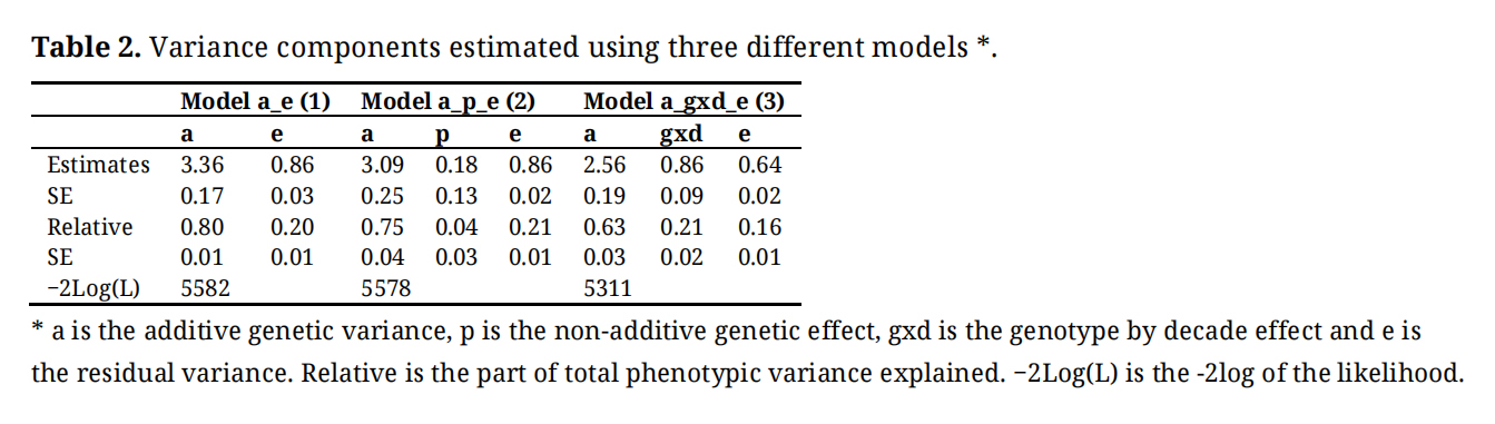Table 2. Variance components estimated using three different models *.

The estimated variance components for LB resistance assessed in different decades from model (4) are presented in Table 3. The phenotypes of the 1980s and 1990s were not included because only few records were available. The estimates of the additive variance and of the residual variance are different across the decades showing a clear decline from first to last decade. The lowest heritability estimate was observed for LB10, corresponding to the resistance challenge done in the 2010s. In contrast, the heritability estimates for LB00 and LB20 were both at 0.86.

TABLE 3

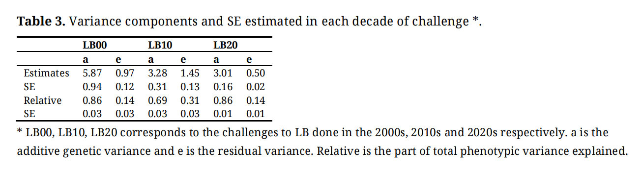Table 3. Variance components and SE estimated in each decade of challenge *.

The genetic correlations between the resistance traits measured across different decades of challenge are presented in Table 4. The correlation ranged from 0.57 to 0.91, with LB00 and LB10 showing the highest correlation. While LB10 and LB20 also showed a high correlation, they may still be considered as distinct traits. The genetic correlation between LB00 and LB20 appeared relatively small compared to the other pairs. This observation corroborates the presence of significant genotype-by-decade interaction.

TABLE 4

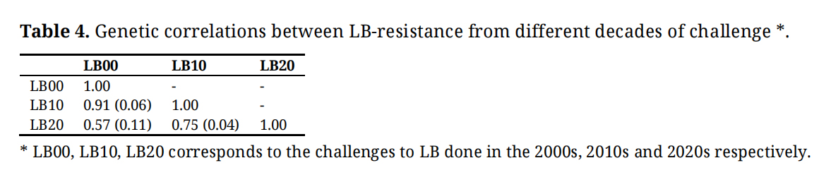Table 4. Genetic correlations between LB-resistance from different decades of challenge *.

Three chromosome regions significantly associated with LB resistance were found and results are summarized in Table 5. The genome regions with significant effects on LB resistance are located on chromosomes 5, 9 and 1.

TABLE 5

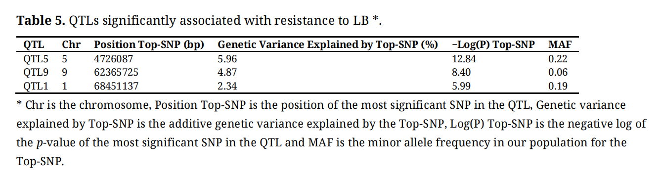Table 5. QTLs significantly associated with resistance to LB *.

TOP-SNP are defined here as the most significant SNP in a genomic region defined as a QTL. We determined that there were 3 chromosome regions with significant effects on LB resistance so there were three TOP SNP, one on chromosome 5, one on chromosome 9, and another SNP on chromosome 1. Even though the QTL on chromosome 5 is known to be linked with maturity [26] we also looked at its effect on LB. Each of the QTL explained 5.96, 4.87 and 2.34 percent of the total additive genetic variance in LB-resistance, respectively.

The effects of different number of alleles in each of the TOP-SNPs are shown in Figure 1. In the population studied, the number of copies of the minor allele of Top SNP of QTL5 on chromosome 5 confers a negative impact on resistance to LB with a clear additive dosage effect. For Top SNP of QTL9 an increased number of copies of the minor allele leads to increased resistance to LB which also seems to be a dosage effect were having one more of the alternate allele confer higher resistance to LB. The alternative allele of Top SNP of QTL1 seems to confer advantages for resistance to LB, where all heterozygous clones have an increased resistance to LB and the gene, therefore, appear to be dominant. No clones were homozygous for the alternative allele. However, it is complicated to draw conclusion on the effects of the number of alleles on the raw phenotype because of the low frequencies of the genotypes with at least three copies of the minor allele. In this population, the frequency of the beneficial allele was 0.78 for the Top-SNP of QTL5, 0.06 for the Top-SNP of QTL9 and 0.19 for the Top-SNP of QTL1.

FIGURE 1

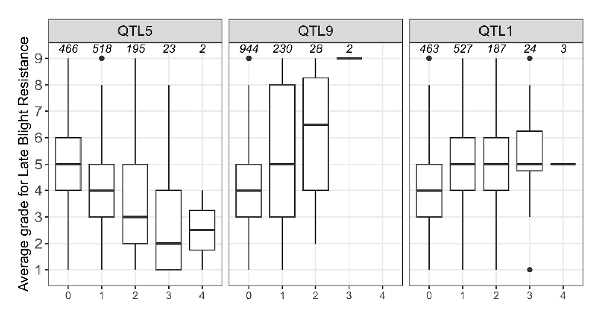Figure 1. Boxplot of phenotype at identified QTL *; * On the x axis are the genotypes (number of alleles of the minor allele) at the TOP-SNP and on the y axis is the average phenotypic value for all individual genotypes. On the top of each box is the number of clones with this specific genotype.

The results of cross validation of models for prediction of breeding values are presented in Table 6. The prediction accuracies evaluated as the correlation between y_c and EBV_reduced ranged from 0.56 to 0.75. Accuracies were similar when using PBLUP, GBLUP or QTL-PBLUP but were markedly higher for the QTL-GBLUP model. The inflation of the distribution of predicted breeding values ranged from 0.91 to 1.32. Overall, for all the models the breeding values were deflated except for the GBLUP where they were inflated.

The correlation between EBV_full and EBV_reduced ranged from 0.70 to 0.90. Accuracies were similar when using PBLUP or QTL-PBLUP but were higher for the models where genomic information was included and especially for the QTL-GBLUP model. The regression indicating dispersion of the predicted breeding values ranged from 0.96 to 1.18.

When associated with the genomic relationship matrix, adding Top-SNP of the three QTL identified as fixed regression into the model led to a considerable gain in accuracy. While no gain was observed when PBLUP and QTL-PBLUP model were compared.

TABLE 6

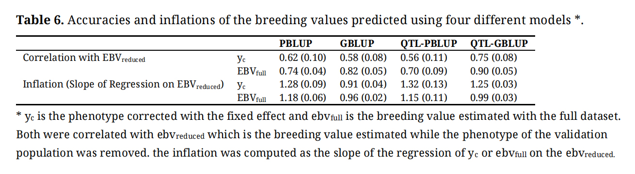Table 6. Accuracies and inflations of the breeding values predicted using four different models *.

Predicted breeding values from model (3), where a genotype by decade interaction effect has been included in the model were used in investigating the genetic trend for LB resistance. Only a few varieties created in the early years of the breeding program had been tested for LB resistance. It is also important to note that some of the varieties presented were included in the test in several years. Indeed, the varieties used as spreader rows have been used across many years, like for example the Bintje variety which has been used over all the 36 years. Moreover, many varieties have related varieties which have been tested as well, leading to more accurate breeding values for these clones.

The estimated genetic trends for LB resistance are shown in Figure 2. No clear trend in the breeding values was observed. It does not seem like there has been any efficient selection for LB resistance as the mean did not change significantly. However, there is an increase in variation of the breeding values with time and we see an increase in number of more resistant (fully or not) varieties from the 2000s with an acceleration from 2010.

FIGURE 2

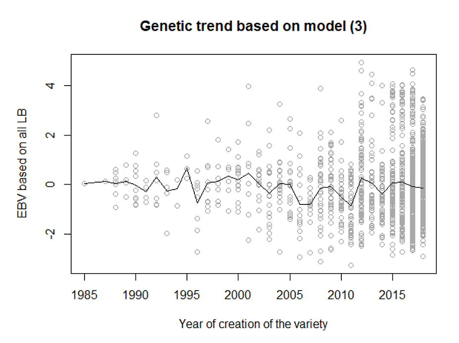Figure 2. Genetic trend for LB resistance *。* Points are the breeding values estimated using model 3 for each of the varieties. Line is the average breeding value per year of first appearance in the breeding program.

DISCUSSION

The comparison of the univariate models gave very strong support for model (3), which includes a genotype by decade interaction that accounts for 21 percent of all phenotypic variance in LB resistance. This significant contribution of genotype-by-time interaction to LB resistance variance has been previously reported [24]. The literature reports a wide range of heritability estimates for LB resistance from 0.31 to 0.85 [22–25,35]. Several factors could explain this variability, such as differences in test procedures and trait definition, in the plant material tested, in the pathogens used for inoculation, or in the methodology used for estimating variance components. In this study the estimated narrow sense heritability defined at the single plot level is very high (0.63) providing a solid basis for selection for resistance towards Pi based on general polygenic breeding values. However, the considerable amount of genotype by decade interaction suggests that resistance could fluctuate over time, potentially due to evolution in the disease agent or due to selective breeding in the tested varieties. A stronger focus a specific pool of parents may also have contributed to the decrease in genetic variance over time. Similar results were found by [24], who found significant genotype-by-year interaction even when experiments were conducted over a much shorter time span than our study. However, yearly effects tend to be strongly affected by differences in weather from year to year, an effect that is expected to be limited when decades are considered. LB resistance measured across different decades shows very high heritability within each decade, but the genetic correlations between resistance in different decades are significantly lower than unity, particularly between the 2020s and earlier decades. This likely reflects a change in the Pi pathogen, rather than the varieties themselves, since limited selection for LB resistance appears to have occurred in the population. In our study, data collection spanned from the 1980s to 2023, with at least seven different Pi pathotypes identified in Denmark between 2006 and 2022 [28]. This means that resistance may reduce or break down due to evolution in Pi. However, the model used to predict breeding values includes a genotype by decade interaction and this provides breeding values averaged over all the decades/years involved and this is expected to provide a more general resistance that is not easily circumvented by the Pi. The estimate of additive genetic variance and especially the estimate of residual variance reduced over the decades investigated. Genetic and environmental variances decreased over time and genetic correlations between distant decades were significantly lower than unity. Again, this indicates a change in the Pi genotypes evolved as there are strong genetic links between clones tested in different decades. However, genetic correlations were sufficient to ensure lasting genetic response for LB resistance. One of the limitations in our study was the scarce amount of data registered in the early years of the breeding program. Acquiring more data per year could help to dissect the genotype by decade interaction, as several factors could have contributed to the interaction. Furthermore, in future testing, a thorough characterization of Pi genotypes involved would be of considerable interest, potentially combined with specific testing of resistance toward well characterized Pi genotypes.

The absence of genetic trend (Figure 2) implies that selection for LB resistance has been limited during the period studied. As previously discussed, this might result from sequential phenotypic selection and/or because of the use of old material as parents in later years. Resistance development has relied heavily on R-genes, which has been utilized since the introgression of R-genes identified in wild potatoes from South America. However, the R-genes are not always a source of long-lasting resistance [9,36]. For example, the pathotype EU_41_A2 acquired the ability to overcome the resistance coming from several R-genes [36]. One proposed strategy has been to accumulate more than one R-genes in a single variety, which is the pyramiding of R-genes approach [14]. In theory, if a single clone carried the beneficial allele for four R-genes, it would become virtually fully resistant to the pathogen targeted [18]. However, this implies for that all the R-genes are 100% effective, which is likely unrealistic [18]. In this study only a few genomic regions affecting LB resistance were identified. This could be because only few resistance genes were present in the population or because they are not effective in the population studied. The latter reason seems most likely as it takes many generations to make a tetraploid population homozygous for a resistance allele.

The three QTL identified in this study explained all together 13% of the additive genetic variance for LB resistance. It means that most of the additive genetic variance in LB resistance is due to the polygenic background, i.e., genes with small effects that cannot be individually identified in our data.

One challenge in selection for LB resistance, is that the loci having a positive effect for resistance may lead to a negative response for other traits of interest. This could explain the low allele frequency of the positive allele for LB resistance for QTL9 and QTL1. For example, the pleiotropy associated with a region on chromosome 5, which affects both maturity and LB resistance, is well-documented [26]. To address this, multi-trait evaluation models should be developed to estimate and exploit genetic correlations between traits, and appropriate economic weights should be assigned to account for potential unfavorable correlations between traits of economic importance. Cloning of the genes involved would also aid in the management of LB resistance.

The accuracy of breeding values predicted from pedigree information or from genomic information was very high. This is not surprising due to the high heritability of LB resistance observed and because most varieties will have many relatives that were also tested. Because of this resemblance between the training and the validating population, a high prediction accuracy is expected. The advantage of using a GBLUP model is relatively limited because of the high heritability of LB resistance and because of the cross-validation strategy which also yielded high accuracies with PBLUP. However, in forward prediction of breeding values for new crosses with few or no close relatives tested a greater advantage of GBLUP model is expected. Moreover, we had access to a deep pedigree allowing accurately tracking the history of the population. The correlation between EBV_full and EBV_reduced indicates the relative change in accuracy when a clone is having its own phenotype removed. The drop in accuracy is relatively small especially for the GBLUP model. This means that if a line is genotyped it is possible to accurately predict its LB resistance before testing this line for LB resistance. Enciso-Rodriguez et al (2018) [24] has drawn the same conclusion from their study. This situation provides excellent possibilities for early selection for LB resistance based on such a combined model. Such a model would lead to a stratified testing of new (and older) clones to update the training population and the use of intense selection among all genotyped individuals. Moreover, the QTL-GBLUP model show that while having own phenotype, genomic information does not improve accuracy of prediction for LB resistance, but incorporating extra information on the genetic architecture of LB resistance could be highly relevant. These results must be interpreted with some caution as the QTL were identified on the entire population, which is also the training population, and this may tend to provide too optimistic results, even though the effects were estimated in the training population only. Even though clear genotype-by-year interaction was observed, selection for LB resistance is still expected to have a lasting effect but continuous testing for LB resistance is needed to identify lack of resistance toward new Pi strains.

CONCLUSIONS

The narrow sense heritability of resistance to LB in potato was large and this shows that results of resistance tests can be used for efficient selection for LB resistance. The resistance changed over time as reflected in a significant interaction between genotype and decade of testing, an interaction that most likely is due to evolution in the Pi. However, the genetic correlation between resistance in different time periods is still substantial so that selection effects will be persistent but potentially will reduce over time. Consistent testing of new lines for resistance is therefore needed. A GWAS study identified three genomic regions that affected resistance toward LB. In total these genomic regions explained 13% of the additive genetic variance in LB resistance. I.e., most of the genetic variance in LB resistance is polygenic and obviously all genetic variation should be used in selection for LB resistance. Extending models so that both identified genomic regions and polygenic variation were used in predicting breeding values clearly yielded the most accurate selection criteria.

DATA AVAILABILITY

The dataset of the study is available from the authors upon reasonable request and will include a confidentiality agreement because the data belongs to an active breeding population.

AUTHOR CONTRIBUTIONS

Conceptualization, HR and JJ; methodology, HR and JJ; formal analysis, HR; data curation, HR; writing—original draft preparation, HR; writing—review and editing, HR, MB and JJ; project administration, HR; funding acquisition, JJ and MB. All authors have read and agreed to the published version of the manuscript.

CONFLICTS OF INTEREST

MB are employed by Danespo A/S, but all authors declare that they have no conflicts of interest.

FUNDING

The project RESPOT was funded by Ministry of Food, Agriculture and Fisheries of Denmark under the Green Development and Demonstrations Program (grant no. 34009-20-1643).