Location: Home >> Detail
J Sustain Res. 2026;8(3):e260077. https://doi.org/10.20900/jsr20260077
 ,
Amanullah Quamer 2 ,
Joshua M. Pearce 1,3,*
,
Amanullah Quamer 2 ,
Joshua M. Pearce 1,3,*
1
2
3
*
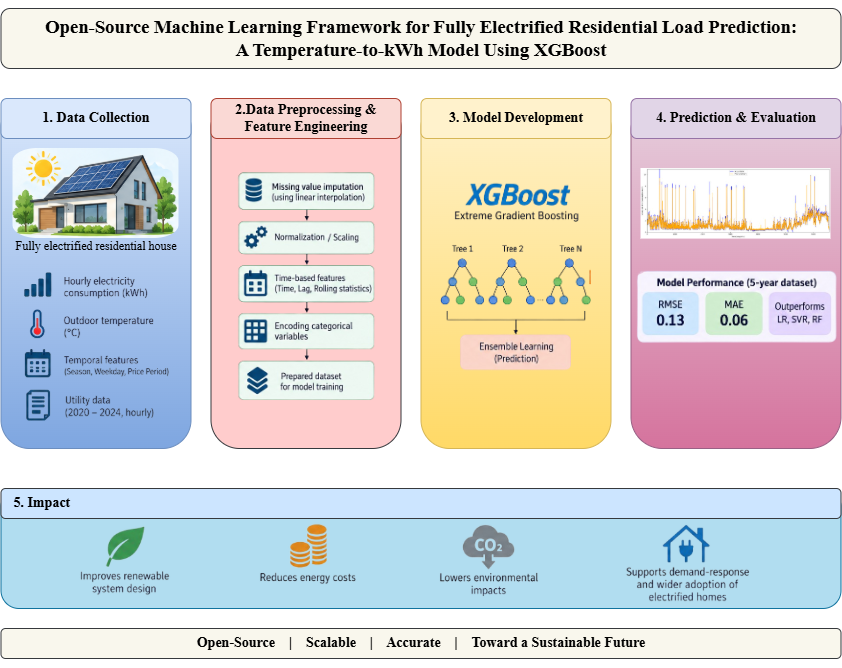
The accelerating shift toward renewable electrification of housing, demands accurate household energy forecasting for optimizing system design, lowering costs and environmental impacts, and optimizing demand-response. To overcome the limitations of existing models, in this study, an open-source, scalable temperature-driven extreme gradient boosting (XGBoost) algorithm model is developed to predict temperature-to-kWh for residential houses. The model captures nonlinear feature interactions and works efficiently with sparse, noisy data. It is trained and validated using a five-year dataset combining hourly household electricity consumption data from a fully solar-powered and electrified residential house in Toronto Canada. The system had solar photovoltaics, photovoltaic thermal and heat pump subsystems. The results showed the novel XGBoost configuration outperformed baseline methods such as linear regression, support vector regression, and random forest and yielded accuracy comparable to or better than reported deep-learning implementations (e.g., multivariate long-short term memory) for similarly sized residential datasets. The results for the model trained with 5-year datasets show RMSE of 0.13 and MAE of 0.06 with the spike handling process, which reflects the model’s reliability for fine-grained residential energy forecasting. This new model can be used to improve optimization and modelling tools to enable a wider deployment of solar-powered fully-electrified residences.
ANN, artificial neural network; HP, heat pump; LR, linear regression; LSTM, long-short term memory; MAE, mean absolute error; MSE, mean square error; PV, photovoltaics; PVT, photovoltaics thermal; kWh, hourly electrical consumption in house; RF, random forest; RMSE, root mean square error; Solar PV, solar photovoltaics; SVR, support vector regression; TCN, temporal convolutional network; XGBoost, extreme gradient boost. Cf, Categorical features; Clag, kWh lag function; Cr, kWh rolling function; Css, Column sample; d.o.w, Day of week; Dmax, Maximum depth of each tree; Entr, Number of decision trees; h, Hours of day; i, Data points; k, Indexing over trees; η, Learning rate; N, Number of; n, Number of iterations; Rt, Rolling temperature; Rs, Random state; Ss, Subsample; t, Time; tr, Tree; ∆T, Temperature difference; yi, Actual observed data points; ŷi, Updated predicted data points; ŷi(n), Prediction at iteration n; ŷi(n−1), Prediction from previous iteration
Anthropogenic energy use is the primary cause of the climate change crisis [1]. The major energy sources are oil products (40.1%), electricity (21.2%), natural gas (16.4%), and coal (8.6%) [2]. The electricity, however, is also generated by burning coal (35.5%) and natural gas (22.1%) [2]. This makes the carbon fuels of coal (45%), oil (33%), and natural gas (21.8%) the largest sources of carbon emissions in world, which emphasizes the need of decarbonization. In recent years, renewable energy resources have emerged as a viable solution [3]. Among renewables, solar photovoltaics (PV) technology has shown unprecedented growth worldwide and has achieved the lowest levelized cost of electricity in history [4]. It is predicted that by the end of this decade solar PV will become the world’s largest source of renewable generation [4]. Although this shift represents a significant step toward reaching climate change objectives, advancements have been unequal in the energy sector. For example, the building sector worldwide consumes 30% of energy (21% for residential alone) and creates 26% of energy-related emissions [5]. Generally, thermal loads represent a major share of residential energy demand, particularly space heating (53%) and hot water demand (16%) however, the relative contribution of heating, cooling, lighting, and other end uses varies with climate, building characteristics, and occupant behavior [6]. In cold climates such as Canada, space heating represents a particularly important component of residential energy demand, and a substantial portion of this demand is still supplied by fossil fuels [6]. In Canada, the residential total final consumption depends heavily on natural gas (42%). Increasing electrification in the residential sector with high-efficiency heat pumps (HP) [7,8] can offer a pathway to sustainably supply thermal loads [9,10]. When HPs are coupled with solar PV [11,12], the solar electric heating systems present a workable solution to cut emissions and eventually reduce the dependency of heating propane and natural gas [13,14]. It can also increase the PV self-consumption and self-sufficiency [15].
As a result of this shift toward renewable and electrified systems, accurate household energy forecasting becomes essential for optimizing system design, lower economic as well as environmental load, and demand-response operations [16–18]. Accurate prediction of household electricity consumption also enables policymakers to design cost-effective retrofit measures, assess long-term economics, and reduce peak-load stress on the grid [19]. Prediction models can be used as tools for estimating and comparing the energy use and efficiency measure in retrofits, helping to achieve the best performance and conservation methods [20,21].
The common approaches for developing these predictions are using physical models, which are covered in detailed reviews [17,22–24]. The disadvantages of these models include the need for specialized expertise, being time-intensive, challenges in the need for precise assumptions, and difficulty to adapt to socio-economic and environmental conditions [25]. These limitations can be overcome by using hybrid models, which combine the physical and data-driven approaches for simulating the building load [17]. The hybrid models, however, face high computational complexity and challenge for properly integrating both physical and data-driven components [26]. Traditional linear approaches to data-driven approaches such as autoregressive models and multiple regression often fail to capture nonlinear interactions between energy use and temperature fluctuations [27,28].
Unlike the physical models, data-driven models do not require detailed information and understanding of the building [29]. This latter approach has gained popularity in the recent year as the proper selection and validation of datasets can ensure prediction accuracy as well as can capture the non-linearity and patterns, but they also require large amounts of data to train the models [24]. The data-driven models use historical datasets and machine learning (ML) algorithms to train [29]. Among the various drivers of household energy demand, ambient temperature remains the most dominant external variable which directly influences heating, cooling, and ventilation requirements [30,31].
The existing literature presents several techniques to forecast residential consumption patterns using temperature and weather variables [32–34]. ML-based approaches such as support vector regression (SVR), random forests (RF) and artificial neural networks (ANN) have shown significant improvement in predictive accuracy by modelling nonlinear dependencies, however, these approaches often underperform when there are random demand spikes that suddenly increase the consumption that are not temperature dependent [35]. Such events typically arise from unpredictable occupant activities such as appliance scheduling or short-term events that leads to increased model variance and degraded generalization [36]. Recently, deep learning models such as long short-term memory (LSTM) networks and temporal convolutional networks (TCN), have been used to model temporal dependencies and long-range correlations [37]. Despite their success in sequence modelling, these architectures are computationally intensive, require extensive labelled data and often suffer from overfitting in small-scale residential datasets [38,39]. However, nonlinear relationships do not necessarily require complex machine-learning models, and simpler statistical or regression approaches can perform competitively depending on the dataset, feature set and forecasting horizon [40].
To overcome the limitations of existing models, in this study, an open-source, scalable temperature-driven extreme gradient boosting (XGBoost) algorithm model is developed to predict temperature-to-kWh for a residential house, which captures nonlinear feature interactions and works efficiently with sparse, noisy data. The model is trained and validated using a five-year dataset (2020–2024) combining hourly household electricity consumption data from a residential house in Toronto Canada, with temperature readings from the National Solar Radiation Database (NSRDB) [41]. By extending the training period from two to five years, the framework systematically evaluates how temporal expansion influences model generalization and introduces spike handling mechanism. A detailed methodology of the proposed model is presented in Section Methodology whereas the results are compared to existing models in literature and discussed in Section Results and Discussions and finally the conclusions are drawn in Section Conclusions.
An overview of the detailed methodology to develop the XGBoost model from ambient temperature for residential house load prediction is shown is Figure 1.
 Figure 1. Overview of the methodology.
The predication model developed in this study uses hourly total electrical energy consumption of a fully electrified residential house located in Toronto, Canada. The house is two stories with a basement and is occupied by two people. The main electrical load comes from the heat pump (2.5-ton and 1.5-ton), induction stove, EV level 2 charger, water heaters, and clothes dryer. The house has a 5 kW of solar photovoltaics (PV) connected to grid through microFIT program [42] (i.e., all the PV electricity generated is sent to grid rather than being used at the site based on a guaranteed fixed feed-in tariffs) and one solar photovoltaics thermal (PVT) module used to pre heat the water for buffer tank that supplies heating and domestic hot water. The historical datasets of the house from January 2020 and December 2024 of the house are used to train the model, which is obtained directly from the electric utility bills. The available electrical dataset of the house is combined with temperature data [41] and has raw input variables (Table 1). Figure 2 shows the simplified schematics of the house. The importance is given to the overall energy consumption in house.
Toronto is considered as the study location because of the high population density [43] and realistic climatic profile for urban Canada, which includes a wide range of temperature fluctuations throughout seasons [44]. According to 2021 census, the population of city of Toronto (Census sub-division) is around 2.79 million which is greater than the sum of four Canadian provinces (i.e., Newfoundland and Labrador, Prince Edward Island, Nova Scotia, and New Brunswick at ~2.6 millions) [45].
 Figure 2. Simplified schematics of the house.
 Table 1. Input variable from raw datasets.
First, the datasets are preprocessed to check for any irregularities and missing values. The missing recorded data points are interpolated by replicating similar hourly trends from neighboring weeks (October 1–15 and November 1–15, 2024). Figure 3 shows the recorded data and interpolated gap for the year 2024. Secondly, data is prepared using Python (v.3.11) [46] with Pandas (v.2.2) [47] and NumPy (v.1.25) [48] to ensure the input features for the model are compatible with each other in terms of time alignment, missing values handling, and numerical compatibility.
 Figure 3. Recorded data and interpolated gap for year 2024.
Step 1. Timestamp alignment
The timestamps recorded under the variable INTERVAL_END_TIME are converted into Python datetime objects to ensure consistent temporal indexing. After conversion, the dataset is chronologically sorted, and the Datetime column is set as the primary index for time-series analysis.
Step 2. Handling missing and inconsistent values
Rows with missing kWh or temperature data are dropped, and small data gaps are interpolated using hourly forward-fill to maintain sequence continuity. All corrections are cross-checked against time indices to ensure integrity.
Step 3. Encoding categorical variables
To enable compatibility with the XGBoost model, categorical features are encoded into numerical forms. Each encoding scheme signifies an ordinal or behavioral distinction relevant to residential energy consumption (Table 2).
 Table 2. Numerical form for each categorical feature.
To capture temporal dependencies, behavioral effects, and lag relationships between temperature and consumption, four new features are introduced in this model using the available datasets. These included time-based, trend-based, lag-based predictors, and behavior flags.
Feature 1. Two-time-based features are extracted directly from the datetime index:
●
●
Feature 2. Trend-based temperature
To incorporate short-term thermal dynamics and capture the temperature transitions effect on load response, differential and rolling temperature metrics are computed. The temperature difference (Equation (1)) is used to quantify the rate of change in ambient temperature between consecutive hours, acting as an indicator of heating or cooling momentum. Whereas a three-hour rolling mean temperature using Equation (2) is obtained to smooth transient temperature variations and represent the short-term environmental trend.
where Rt is the rolling temperature (T) at time t, ∆Tt is the temperature difference at t, and h is hour.
Feature 3. Consumption lag and rolling average features
Energy usage inherently depends on previous consumption states [49]. Therefore, one, two and three hour lagged kWh values are added in the model using Equation (3). In addition, a three-hour rolling average of kWh is computed to provide a smoothed representation of recent energy usage (Equation (4)).
where, Clag(t) is lagged kWh which provides a direct measure of load inertia at time t, while Cr(t) is the rolling kWh used to stabilize short-term fluctuations, creating a smoother contextual input for the regression model.
Feature 4. Behavioral flags
Human activity strongly influences energy usage in the house [50]. Hence, binary variables for weekends, holidays, and seasons are introduced to reflect occupancy-related behavior changes. Each feature is standardized to compatible numeric scale and validated for correlation stability before model training.
After defining the features, the datasets are partitioned chronologically to emulate real-world forecasting conditions and to minimize the risk of temporal data leakage, which is a common issue in time-series prediction models [51]. Unlike a conventional random train-test split, random partitioning of time-dependent observations can place future observations in the training set while earlier observations are assigned to the test set. This can introduce look-ahead bias because information from periods occurring later in time may indirectly influence model fitting and lead to an overly optimistic estimate of predictive performance. To avoid this issue, the data were ordered chronologically, and each test period was restricted to observations occurring after the corresponding training period. Three progressively expanding training configurations were therefore constructed as Set 1 (2020–2021), Set 2 (2020–2023), and Set 3 (2020–2024). For each modelling setup (Table 3), 85% of the available observations were used for model training and the remaining 15% were retained as a temporally subsequent test set. For reproducibility, the number of observations used in each training and testing configuration is also reported. The exact sample counts were obtained after timestamp alignment, missing-value processing, and feature construction, and therefore correspond to the final datasets supplied to the XGBoost model rather than the nominal calendar duration alone. This design allows the model to be evaluated only on data that would have been unavailable during training, while also examining how increasing the historical training horizon affects predictive performance.
 Table 3. Training configurations for each modeling phase.
The XGBoost algorithm is chosen as the main regression framework in this study to model nonlinear interactions between mixed numerical and categorical variables efficiently. The proposed framework builds an ensemble of decision trees in each step. Each new tree focuses on fixing the mistakes made by the previous step, which optimizes prediction of accuracy. The proposed model uses a regularized objective function (Equation (5)) designed to balance predictive performance and model complexity. The additive update rule for each boosting iteration is obtained using Equation (6).
where, L(∅) is the total loss function which the model tries to minimize during training, l(yi, ŷi) denotes the mean-squared-error (MSE) loss between predicted and observed values, and Ω(fk) is a regularization term that penalizes overly complex trees to prevent overfitting. Whereas i is index over data points, yi is actual observed kWh and ŷi is updated predicted kWh, k is indexing over trees fk is kth tree in the model which tries to correct errors from earlier trees, ŷi(n) is prediction at iteration n, ŷi(n−1) is prediction from previous iteration, ftr(xi) is output of the new tree for input xi which adds correction value to fix previous prediction errors, and η is the learning rate that controls how much each new tree ftr adds to the model. The model learns slowly and efficiently across different consumption patterns as it uses combination of regularized loss and gradient-based additive boosting. The tuned parameters used in model and their function is presented in Tables 4 and 5.
 Table 4. Input tuned parameters for XGBoost model.
 Table 5. Function of tuned parameters.
During exploratory analysis, the energy data displayed irregular high-magnitude consumption spikes unrelated to temperature. To improve resilience, a spike correction post-processing step is introduced in this study. A spike threshold τ = 6 kWh is empirically determined based on mean ±1.5σ of kWh values. If the predicted consumption (ŷi) is below 1 kWh while the actual exceeded τ, the prediction is replaced with the actual to avoid severe underestimation (Equation (7)).
finally, the performance of the developed XGBoost is evaluated based on the standard regression metrics i.e., root mean squared error (RMSE) and mean absolute error (MAE) using Equations (8) and (9), respectively. N is the total number of test samples, (yi − ŷi)2 is squared error for each prediction, penalizing larger mistakes more heavily, |yi − ŷi| is absolute prediction error at each time step, and M is number of predictions evaluated.
Initial inspection of raw datasets revealed approximately 43,800 hourly entries across the five-year study period, with missing records amounting to less than 1% (372 hourly intervals were missing in October 2024). Figure 4 shows the interpolated data points for the missing values. The timestamp alignment ensures that each hourly observation is properly sequenced, and no overlapping or unordered timestamps remain in the dataset. Whereas data handling approach keeps the autocorrelation structure of the series while avoiding artificial distortions that might arise from global interpolation techniques. The use of encoding categorical variable enables the model to perceive discrete scheduling and pricing periods as significant predictors of consumption patterns. In particular, the weekday flag captured behavioral differences in household consumption use between working days and weekends, while price period shows potential demand-shifting behaviors influenced by time-of-use tariffs.
 Figure 4. Interpolated gap and data points data for year 2024.
Secondly, feature engineering, i.e., time-based features (Feature 1), help the model recognize intra-day and intra-week consumption cycles, i.e., higher energy use during early morning heating or evening appliance usage periods. This inclusion allows XGBoost to implicitly learn the recurring temporal demand structure present in hourly residential consumption data. Trend based features (Feature 2) using Equation (1) effectively filters noise from high-frequency fluctuations (e.g., transient thermal spikes), while Equation (2) enhances the model’s responsiveness to rapid thermal transitions, both of which are critical for understanding HVAC-driven energy variability. Consumption lag and rolling (Feature 3) together are used in the model to learn sequential dependencies which mitigate the effects of random consumption spikes. Behavioral flags (Feature 4) balance short-term load persistence with external thermal sensitivity as they use lag, trend, and behavioral features to give an accurate view of energy flows in homes. The processed input features used in the XGBoost model are shown in Table 6.
 Table 6. Processed input features for XGBoost model.
This section presents the experimental outcomes of the proposed temperature-to-kWh prediction model based on the XGBoost regression framework. The selection of XGBoost was motivated by the structured combination of numerical, categorical, temporal, and lag-based predictors used in this study. XGBoost can capture nonlinear interactions among these features while using regularization to control model complexity and reduce overfitting. These characteristics make XGBoost suitable for the relatively structured residential dataset investigated in this study. The results are shown in sequence from earliest to latest which shows how gradually increasing the training horizon from a two-year baseline (2020–2021) to expanded datasets with four years (2020–2023) and five years (2020–2024) affects the outcomes. The outcome of each training set is post-processed using spike correction to enhance the spike alignment and reduced underprediction bias. Finally, the model accuracy is evaluated using the RMSE and MAE values which is supported by qualitative assessment of the temporal alignment between actual and predicted electricity consumption curves.
Baseline Performance: 2020–2021 DatasetThe initial training used two years of data (January 2020 to December 2021) i.e., set 1 to establish a baseline model. The XGBoost regressor achieved an RMSE value of 0.48 which indicates moderate predictive accuracy when trained with a limited dataset. Figure 5 shows the comparison between the actual and predicted hourly kWh consumption for the test period (October–December 2021).
 Figure 5. Actual and predicted kWh using XGBoost model for year 2020–2021 (Set 1).
The results show that model trained with set 1 successfully captured the general consumption trends, including daily periodicity and temperature-driven variations. Whereas certain random consumption spikes which were caused by non-temperature factors such as occupant behavior or appliance operations, are only partially detected. Set 1 model, however, cannot generalize across random spikes because of the concise training data. Nonetheless, the model maintained temporal coherence, with prediction lags of less than two hours during abrupt temperature transitions. The baseline experiment thus establishes the learning capacity of XGBoost in a purely temperature-driven framework which serves as a reference for subsequent multi-year models.
Extended Training Horizon: 2020–2023 DatasetTo enhance the model’s generalization over the dataset, the training horizon is extended to four years cycle (2020–2023) i.e., set 2. This allowed the model to fetch broader climatic variations and behavioral cycles which include seasonal load patterns across multiple winters and summers. The retrained model shows good improvement with an RMSE score of 0.27, which is a 43% reduction compared to the baseline model. Figure 6 shows the alignment between predicted and actual kWh consumption for the last quarter of 2023. The model effectively reproduced both day-time fluctuations and temperature-correlated peaks with improved spike sensitivity relative to the baseline model. Overall, the model's trajectory closely matched observed data, even though some underestimation continued during high-load hours, especially in early morning heating cycles.
The performance improvement in the second training is because of increased data pattern from multiple seasonal cycles, lag and rolling features which are introduced in preprocessing, and feature-temperature coupling achieved by the gradient-boosting architecture. The second set model also demonstrated higher stability with less noise adjustment in flat-load periods as compared to shorter training windows (set 1). These findings confirm that longer temporal exposure enhances model robustness and reduces overfitting to short-term fluctuations.
 Figure 6. Actual and predicted kWh using XGBoost model for year 2020–2023 (Set 2).
The final and most comprehensive model which includes five years of training data i.e., set 3 (2020–2024), after addressing data discontinuities in October 2024, where around 16 days of hourly intervals were missing. The missing 372 records (~4.2% of annual data) were reconstructed using temporal interpolation as illustrated earlier in Figure 4 of Section Processed data. This ensured consistent input resolution for training. After retraining with the complete five-year dataset, the XGBoost model achieved an RMSE score of 0.13 which marks a 73% and 52% improvement as compared to the baseline model (set 1) and four-year (set 2), respectively. Figure 7 shows the corresponding actual and predicted consumption trends for the last quarter of 2024.
 Figure 7.
Actual and predicted kWh using XGBoost model for year 2020–2024 (Set 3).
Figure 7.
Actual and predicted kWh using XGBoost model for year 2020–2024 (Set 3).
The model demonstrates closeness with the recorded kWh trajectory i.e., precise reproduction of sharp consumption peaks. The spike-handling mechanism implemented using np.clip() and conditional correction methods proved to be highly effective in decreasing unrealistic overpredictions while keeping important high-load events. Set 3 training model also maintained numerical stability under high-temperature changes and captured inter-day oscillations driven by weekday to weekend transitions. Error analysis shows that MAE value of 0.06 kWh, which confirms the model’s reliability for fine-grained residential energy forecasting. The stability between feature importance across training iterations further supports robustness of the model with temperature, lagged consumption, and short-term thermal momentum (Rt) emerging as dominant predictors.
Comparative Evaluation and Feature InterpretabilityThe progressive improvement in proposed model performance across different training horizons with and without proposed spike handling correction is shown in Table 7, which reports the RMSE and MAE values for all three experimental approaches. As the training duration increased, the error consistently decreased which validates the temporal diversity. Whereas the expanded climatic representation substantially enhances generalization. The results from the XGBoost model without proposed spike handling have a RMSE value of 0.48, 0.28, and 0.23 whereas when the post-processing of outcomes are done there is an improvement of 4% and 43% in training set 2 and set 3, respectively. Similarly, the MAE values improve from 0.16, 0.12, and 0.1 to 0.15, 0.11, and 0.06 for training set 1, 2, and 3, respectively. A significant improvement is seen with training set 3 due to large training datasets which provide long-term learning and adaptation. Table 8 shows the comparison of different training sets after the results from proposed models are post-processed using spike correction. The result shows that when trained with set 3, model has an approximate decrease of 73% and 60% in RMSE and MAE value compared to when trained with set 1 which shows the improvement of model and closeness to accuracy. Similarly, when set 3 outcomes are compared with the set 2, there is an improvement of 44% and 27% in RMSE and MAE value respectively.
Additionally, feature importance analysis is performed using the feature_importances_attribute for the trained XGBoost model. The ranking shows temperature, kWhlag and kWhrolling as the most important features, which contribute to more than 70% of total model importance which can be shown in the Figure 8. Behavioral flags such as weekdayflag and priceperiod contribute moderately, which reflect their importance in capturing occupancy-driven variations. The results indicate that temperature is the primary driver of energy consumption, when combined with lagged consumption and engineered temperature-trend features the model better captures sudden demand spike while maintaining stable and smooth short-term predictions. smoothness over short-term volatility.
 Table 7. Evaluation parameters of different sets with/without spike mechanism.
 Table 8. Comparison of evaluation of parameters of different training sets.
 Figure 8. Feature Importance Ranking of XGBoost Model.
The comparative evaluation summarized in Table 9 shows the XGBoost configuration outperformed baseline methods such as SVR, linear regression, and RF on the same problem formulation, and yielded accuracy comparable to or better than reported deep-learning implementations (e.g., multivariate LSTM) for similarly sized residential datasets. These results, however, should not be interpreted as evidence that XGBoost or other trainable models always outperform simpler alternatives. Differences in datasets, input features, forecasting horizons, and evaluation protocols limit direct comparison across studies. Thus, the results support the suitability of XGBoost for the present application rather than establishing universal superiority. The advantage of proposed XGBoost derives from its efficiency on tabular inputs which reduced hyperparameter sensitivity and the ability to naturally incorporate lagged and rolling features without extensive normalization or sequence modeling overhead.
 Table 9. Comparison of proposed XGBoost model with existing models in literature.
The main contribution of this study is the spike-handling mechanism integrated into XGBoost prediction model. Residential load series contain abrupt, high-magnitude spikes that are typically driven by occupant actions, appliance cycling, or one-off events and therefore are poorly explained by temperature alone [56]. The applied methodology in this study, i.e., post-processing rules and clipping logic reduced systematic underestimation of such extreme events, producing closer alignment of predicted peaks with observed spikes. This correction improved the model’s upper-tail fidelity without materially increasing false positives, thereby making the forecasts more actionable for retrofit assessment and demand-response planning.
Limitation and Future WorkDespite these strengths, there are key limitations to this new model. Spikes tied to non-temperature events such as holidays, unexpected occupancy changes, maintenance activities, or tariff-induced behavioral shifts remain only partially addressed because they are not represented in the current input space. Although the spike-correction step mitigates the immediate impact of underprediction during those events, it does not provide explanatory insight nor a predictive pathway for occasions entirely driven by human behavior or operational schedules. A further limitation includes limited training data. The current model was trained and evaluated using data from a single two-occupant residential house in Toronto, which limits its generalizability across different climates, building types, occupancy levels, and residential energy systems. Future work, therefore, should evaluate multi-building datasets spanning diverse climates and household characteristics. Transfer learning could also be explored to adapt the learned relationships from the Toronto dataset to new buildings with limited historical data, while incorporating battery-equipped systems which would further extend the models applicability to different residential configurations. The current feature set also excludes building-envelope thermal performance, indoor heating or cooling setpoints, segmented appliance consumption, and real-time occupancy signals. Future work should include a sensitivity analysis involving these variables which can help quantify their individual contribution to prediction accuracy and distinguish temperature-driven demand from building and behavior-driven loads. This would also strengthen estimation of energy savings and decarbonization benefits associated with retrofit measures. Further, deep learning approaches such as LSTM and TCN were not experimentally evaluated because of their greater computational and sequence-modelling requirements and may require larger datasets for effective training. Another limitation is that the present study does not provide controlled experiments comparing XGBoost with simpler statistical models under identical data and evaluation conditions. Consequently, the observed performance should be interpreted within the scope of the present dataset and feature configuration. Future work should conduct controlled cross-model evaluations to determine when additional model complexity provides meaningful forecasting gains.
To address these limitations, future research could add modelling steps that include smart-meter data with individual appliance-level consumption, household occupancy information, and data from multiple dwellings to understand usage patterns, capture behavioral variability, and improve the generalizability of the model for different locations. Based on these future modelling work can be done in three directions. First, future work can enrich the feature set with contextual indicators (i.e., occupancy proxies, appliance-level signals, smart-meter metadata, and tariff schedules) to enable causal modelling of non-temperature spikes [57]. Second, future research could investigate hybrid modeling that uses XGBoost’s interpretability with sequence learners (i.e., LSTM/TCN) to better capturing long-range temporal dependencies while preserving feature importance transparency. Third, integrating anomaly-detection modules into flag and reducing irregular events differently during training and inference which thereby reduces the distortion of model parameters. Together these enhancements will focus on reducing residual error during high-variability intervals. This will increase the model’s utility for retrofit planning, operational decision-making and scalable deployment in real-world residential settings. Lastly, this model can be integrated into open source energy model simulators/optimizers to better develop both on-grid and off-grid fully PV-powered residences [58,59]. The model can be integrated for PV sizing in [15] as it can predict the hourly electrical consumption which can help estimate the mismatch between demand and supply. Thus, helping with open source home energy management systems and control strategies [60–62] as well as allowing homeowners to optimize both electrical [63] and thermal storage [64,65].
This study presents a novel XGBoost regression model which provides a stable and scalable framework for hourly residential electricity forecasting for fully electrified residences where temperature is taken as the primary external input. The model is trained using three training sets starting from set 1 (2 years datasets), set 2 (4 years datasets), and set 3 (5 years datasets). 85% of the datasets in each training set are used to train the model based on proposed methodology and 15% is used to validate the model. A new spike handling mechanism is proposed in the study for post-processing of the XGBoost model. Finally, the developed model is evaluated based on RMSE and MAE values. The model converged reliably and produced consistent predictions with modest computation. This stability comes from the algorithm’s gradient-boosting architecture, regularization controls and ability to learn nonlinear interactions from engineered features used in the study. These properties enabled robust performance using a relatively small and structured feature set, confirming that tree-based ensemble methods making it highly effective for temperature-to-kWh tasks where interpretability and reproducibility are considered as priorities. The comparative results support the suitability of XGBoost relative to the alternative models considered.
Model performance improved substantially as the available training sets are lengthened i.e., from set 1 to set 3 reduced RMSE indicating that broader temporal exposure allows the model to learn recurrent seasonal patterns, weekday to weekend behavioral cycles, and uncommon but recurring high-demand events. The results show an improvement of 43% and 40% in evaluation parameter with post processing (spike correction mechanism) of the model trained with set 3 compared to without it. The gains from longer training windows show improved coverage of different climatic conditions and usage scenarios which in turn reduce the model variance and increase generalization across unseen periods. The result highlights when model trained with training, set 3 (i.e., 5-year datasets) show RMSE of 0.13 and MAE of 0.06 with spike handling process which reflects the model’s reliability for fine-grained residential energy forecasting and has 73% and 60% improvement compared to training set 1.
The limitation of this study, however, includes partial handling of spike mechanisms which arise due to non-temperature dependent parameters which were not included in feature sets of models. Therefore, future work should (i) include the non-temperature dependent input parameter to capture the random spike (ii) use of hybrid modelling approaches for residential house load prediction, and (iii) integrate anomaly detection module to identify and handle irregular events. These improvements will help increase the reliability and adaptability of the real-world residential settings as well as improve optimization and modeling tools to enable a wider deployment of solar powered fully electrified residences.
All the data and code for this project are available on the Open Science Framework https://doi.org/10.17605/OSF.IO/BWS3Y.
Conceptualization, JMP; methodology, SR, AQ and JMP; software, AQ; validation, SR, AQ and JMP; formal analysis, SR, AQ and JMP; investigation, SR, AQ; resources, JMP; data curation, SR and AQ; writing—original draft preparation, SR, AQ and JMP; writing—review and editing, SR, AQ and JMP; visualization, SR and AQ; supervision, JMP; project administration, JMP; funding acquisition, JMP. All authors have read and agreed to the published version of the manuscript.
The authors declare that they have no conflicts of interest.
This work was supported by the Natural Sciences and Engineering Research Council of Canada and the Thompson Endowment.
The authors would like to thank Paul Dowsett, Founding Architect at Sustainable, for helpful discussions and data access.
1.
2.
3.
4.
5.
6.
7.
8.
9.
10.
11.
12.
13.
14.
15.
16.
17.
18.
19.
20.
21.
22.
23.
24.
25.
26.
27.
28.
29.
30.
31.
32.
33.
34.
35.
36.
37.
38.
39.
40.
41.
42.
43.
44.
45.
46.
47.
48.
49.
50.
51.
52.
53.
54.
55.
56.
57.
58.
59.
60.
61.
62.
63.
64.
65.
Rana S, Quamer A, Pearce JM. Open-Source Machine Learning Framework for Fully Electrified Residential Load Prediction: A Temperature-to-kWh Model Using XGBoost. J Sustain Res. 2026;8(3):e260077. https://doi.org/10.20900/jsr20260077.

Copyright © Hapres Co., Ltd. Privacy Policy | Terms and Conditions


